Lesson 22: Full Backprop Through the Block
15-backpropagation derived the chain rule one layer at a time; 13-transformer-block assembled the forward pass of one block. This lesson wires the two together: the complete analytical backward pass through a Pre-LN single-head transformer block — LayerNorm, scaled dot-product attention, residuals, FFN with GELU, LM head — derived in seven pieces, mapped line by line onto the shared library, verified against a finite-difference probe, and then used to train the block end-to-end on a corpus that a bigram model cannot solve.
The forward/backward pair lives in lib/transformer.rlab (transformer_forward, transformer_backward, adamw_step). It is the engine that the capstone (23-putting-it-all-together) and the fine-tuning lesson (25-fine-tuning-sft-and-dpo) run on, so every line of it is derived here rather than treated as a black box.
Learning Objectives
- Derive the full backward pass through a Pre-LN single-head transformer block in seven pieces — cross-entropy, LM head, residual splits, FFN with \(\mathrm{GELU}'\), LayerNorm, attention with the scaled dot product and mask, Q/K/V projections and the embedding scatter-add — and map each piece to the line of
transformer_backwardthat implements it. - Verify the analytical gradient against a central finite-difference probe and read the ε V-curve: truncation error on one side, floating-point cancellation on the other.
- Train the block to drive the loss below the bigram floor on a context-2 corpus, then ablate attention and the positional code to see which mechanism actually beat the floor.
- Read the backward pass as the adjoint recursion of 15-backpropagation and the bigram floor as a conditional entropy of the corpus.
Background
- Chain rule through every transformer layer from 15-backpropagation — this lesson composes them.
- The transformer block forward pass from 13-transformer-block — used verbatim (single head, with LayerNorm affines and FFN biases).
- AdamW + warmup-cosine training pattern from 16-adamw-optimizer, 17-learning-rate-scheduling, and 18-training-loop.
- Conditional entropy from 05-bigram-language-model; the helpers in
lib/info.rlab.
A Corpus Where Attention Beats Bigram
Theory
To demonstrate that backprop through attention works, we need a task that attention can solve but bigram cannot. The period-3 corpus "abbabbabbabb" (12 tokens, 11 pairs) has exactly this property:
| Context | Bigram says | Truth |
|---|---|---|
After a | always b (P=1) | always b ✓ |
After b (middle of abb) | \(P(b\mid b) = 4/7\), \(P(a\mid b) = 3/7\) | always b ✗ |
After b (end of abb) | same as above | always a ✗ |
A bigram model cannot distinguish the two b contexts. The analytic floor:
\[\mathcal{L}_{\text{bigram}} = \frac{1}{11}\!\left(4 \cdot 0 + 4 \cdot (-\log\tfrac{4}{7}) + 3 \cdot (-\log\tfrac{3}{7})\right) \approx 0.434\ \text{nats/pair}.\]
A trigram (or any model with a 2-token context window) can predict every next token with \(P = 1\), so its loss floor is exactly \(0\). Attention with \(d_{\text{head}} \geq 2\) has enough capacity to encode this context. The trained model should drive the loss from ~0.6 (random init) below the bigram floor of 0.434 toward 0.
Beating the floor shows the model uses more than the current token — but it does not, on its own, prove the extra signal comes from attention. On this short, fixed corpus the model also carries a fixed sinusoidal positional embedding, which makes every one of the 12 positions distinct; the FFN can memorise a position→next-token map with attention contributing nothing. The ablation at the end of this lesson measures exactly that. The decisive evidence that backprop through attention is correct is the finite-difference gradient check, which probes a weight (Wq) that lives inside the attention path.
Example — Corpus and parameters
All trainable parameters travel in one struct P so that the library functions have short signatures. Positional encodings are fixed (not trained). P0 keeps a by-value snapshot of the random initialisation for the ablation later.
seed(24);
vocab = 2;             % tokens: a=1, b=2
d_model = 4;
d_ff = 8;
T_max = 16;

pat = [1, 2, 2];       % a, b, b
T = 12;
ids = zeros(T);
for i = 1:T
  ids(i) = pat(mod(i - 1, 3) + 1);
end
mask = ones(T - 1);    % every prediction position counts

E = randn(vocab, d_model) * 0.3;
PE = sinusoidal_pe(T_max, d_model);
gamma1 = ones(d_model);   beta1 = zeros(d_model);
gamma2 = ones(d_model);   beta2 = zeros(d_model);
Wq = randn(d_model, d_model) * 0.3;
Wk = randn(d_model, d_model) * 0.3;
Wv = randn(d_model, d_model) * 0.3;
Wo = randn(d_model, d_model) * 0.3;
W1 = randn(d_model, d_ff) * 0.3;  b1f = zeros(d_ff);
W2 = randn(d_ff, d_model) * 0.3;  b2f = zeros(d_model);
W_U = randn(d_model, vocab) * 0.3;
P = struct("E", E, "PE", PE, "gamma1", gamma1, "beta1", beta1, "gamma2", gamma2, "beta2", beta2, ...
           "Wq", Wq, "Wk", Wk, "Wv", Wv, "Wo", Wo, "W1", W1, "b1f", b1f, "W2", W2, "b2f", b2f, "W_U", W_U);
P0 = P;
print("tokens:", ids);tokens: [1×12] 1.000000 2.000000 2.000000 1.000000 2.000000 2.000000 1.000000 2.000000 ... (12 total)The Full Backward Pass
Theory
The forward pass through one Pre-LN block is
\[\begin{aligned} \mathbf{H}_{\ln 1} &= \mathrm{LN}_1(\mathbf{H}_{\text{in}}) \\ \mathbf{Q}, \mathbf{K}, \mathbf{V} &= \mathbf{H}_{\ln 1} \mathbf{W}_Q,\; \mathbf{H}_{\ln 1} \mathbf{W}_K,\; \mathbf{H}_{\ln 1} \mathbf{W}_V \\ \mathbf{S} &= \mathbf{Q} \mathbf{K}^\top / \sqrt{d} + \mathrm{mask} \\ \mathbf{A} &= \mathrm{softmax}(\mathbf{S})\quad\text{(row-wise)} \\ \mathbf{H}_{\text{mid}} &= \mathbf{H}_{\text{in}} + (\mathbf{A} \mathbf{V}) \mathbf{W}_O \\ \mathbf{H}_{\ln 2} &= \mathrm{LN}_2(\mathbf{H}_{\text{mid}}) \\ \mathbf{H}_{\text{out}} &= \mathbf{H}_{\text{mid}} + \mathrm{GELU}(\mathbf{H}_{\ln 2} \mathbf{W}_1 + \mathbf{1}\mathbf{b}_1^\top) \mathbf{W}_2 + \mathbf{1}\mathbf{b}_2^\top \end{aligned}\]
with \(\mathbf{H}_{\text{in}}(t,:) = \mathbf{E}(\mathrm{ids}(t),:) + \mathbf{PE}(t,:)\), a single head so \(d = d_{\text{model}}\), and a final LM head \(\mathbf{Z} = \mathbf{H}_{\text{out}} \mathbf{W}_U\) producing the logits. The loss is the masked mean cross-entropy over the counted prediction positions \(\mathcal{T}\) (\(n = \lvert\mathcal{T}\rvert\); here every position counts, \(n = 11\)).
Write \(\bar{\mathbf{X}} = \partial\mathcal{L}/\partial\mathbf{X}\) for the adjoint of any intermediate (00-the-llm-as-a-system; dX in code). Two rules from 15-backpropagation do almost all the work: for a matrix product \(\mathbf{Y} = \mathbf{X}\mathbf{W}\), \(\bar{\mathbf{X}} = \bar{\mathbf{Y}}\mathbf{W}^\top\) and \(\bar{\mathbf{W}} = \mathbf{X}^\top\bar{\mathbf{Y}}\); for an element-wise map \(\mathbf{Y} = f(\mathbf{X})\), \(\bar{\mathbf{X}} = \bar{\mathbf{Y}}\odot f'(\mathbf{X})\). The backward pass is the forward list read bottom-up, one rule per line. Each piece below quotes the line(s) of transformer_backward in lib/transformer.rlab that implement it.
(1) Cross-entropy → logits. For one counted row, \(\ell_t = -\log \mathrm{softmax}(\mathbf{z}_t)_{y_t}\) with \(y_t = \mathrm{ids}(t+1)\), and 15-backpropagation showed \(\partial \ell_t/\partial \mathbf{z}_t = \mathbf{p}_t - \mathbf{e}_{y_t}\). The mean over \(n\) positions divides by \(n\); rows outside \(\mathcal{T}\) (and the last row, which predicts nothing) get zero:
\[\bar{\mathbf{Z}}(t,:) = \begin{cases}(\mathbf{p}_t - \mathbf{e}_{y_t})/n & t \in \mathcal{T} \\ \mathbf{0} & \text{otherwise.}\end{cases}\]
p = softmax(logits(t, :));
e_y = zeros(vocab); e_y(ids(t + 1)) = 1.0;
dl(t, :) = (p - e_y) / total;          % ce_dlogits, lines 227-229
(2) LM head. \(\mathbf{Z} = \mathbf{H}_{\text{out}}\mathbf{W}_U\) is a plain product, so
\[\bar{\mathbf{W}}_U = \mathbf{H}_{\text{out}}^\top \bar{\mathbf{Z}}, \qquad \bar{\mathbf{H}}_{\text{out}} = \bar{\mathbf{Z}}\, \mathbf{W}_U^\top .\]
dW_U = H_out' * dlogits;               % lines 267-268
dH_out = dlogits * W_U';
(3) Residual splits. \(\mathbf{H}_{\text{out}} = \mathbf{H}_{\text{mid}} + \mathrm{ffn}\) is a sum, and the adjoint of a sum is copied to both summands: \(\overline{\mathrm{ffn}} = \bar{\mathbf{H}}_{\text{out}}\) and \(\bar{\mathbf{H}}_{\text{mid}} \mathrel{+}= \bar{\mathbf{H}}_{\text{out}}\). The branch's own contribution to \(\bar{\mathbf{H}}_{\text{mid}}\) is added later, once it has been computed (line 293). The attention residual \(\mathbf{H}_{\text{mid}} = \mathbf{H}_{\text{in}} + \mathrm{proj}\) splits the same way (lines 296–297, 327). This is why gradients cannot vanish through a residual stack: the identity path carries \(\bar{\mathbf{H}}\) back unattenuated.
d_ffn_out = dH_out;                    % lines 271-272
dH_mid    = dH_out;
(4) FFN. With \(\mathbf{U} = \mathbf{H}_{\ln 2}\mathbf{W}_1 + \mathbf{1}\mathbf{b}_1^\top\), \(\mathbf{G} = \mathrm{GELU}(\mathbf{U})\), \(\mathrm{ffn} = \mathbf{G}\mathbf{W}_2 + \mathbf{1}\mathbf{b}_2^\top\), apply the product rule twice and the element-wise rule once. A bias is broadcast to every row in the forward pass, so its adjoint is the column sum over rows:
\[\bar{\mathbf{W}}_2 = \mathbf{G}^\top\overline{\mathrm{ffn}}, \quad \bar{\mathbf{b}}_2 = \textstyle\sum_t \overline{\mathrm{ffn}}(t,:), \quad \bar{\mathbf{G}} = \overline{\mathrm{ffn}}\,\mathbf{W}_2^\top, \quad \bar{\mathbf{U}} = \bar{\mathbf{G}} \odot \mathrm{GELU}'(\mathbf{U}),\]
\[\bar{\mathbf{W}}_1 = \mathbf{H}_{\ln 2}^\top\bar{\mathbf{U}}, \quad \bar{\mathbf{b}}_1 = \textstyle\sum_t \bar{\mathbf{U}}(t,:), \quad \bar{\mathbf{H}}_{\ln 2} = \bar{\mathbf{U}}\,\mathbf{W}_1^\top .\]
The gelu builtin is the tanh approximation \(\mathrm{GELU}(z) = \tfrac12 z\,(1 + \tanh u)\) with \(u = c\,(z + 0.044715\,z^3)\), \(c = \sqrt{2/\pi}\), so by the product and chain rules
\[\mathrm{GELU}'(z) = \tfrac12 (1 + \tanh u) + \tfrac12 z\,(1 - \tanh^2 u)\; c\,(1 + 3 \cdot 0.044715\, z^2),\]
which is gelu_grad (lines 138–145): the first term is the "gate" value, the second is the gate's slope times \(z\).
dhidden = d_ffn_out * W2';             % lines 275-289
dW2 = hidden' * d_ffn_out;
db2f = db2f + d_ffn_out(t, :);         % summed over t
dpre_gelu = dhidden .* gelu_grad(pre_gelu);
dH_ln2 = dpre_gelu * W1';
dW1 = H_ln2' * dpre_gelu;
db1f = db1f + dpre_gelu(t, :);         % summed over t
(5) LayerNorm. Per row, \(\mathbf{y} = \tilde{\mathbf{x}} \odot \boldsymbol{\gamma} + \boldsymbol{\beta}\) with \(\tilde{\mathbf{x}} = (\mathbf{x} - \mu)/\sigma\), \(\mu = \mathrm{mean}(\mathbf{x})\), \(\sigma = \sqrt{\mathrm{var}(\mathbf{x}) + \varepsilon}\). The affine part is immediate:
\[\bar{\boldsymbol{\gamma}} = \sum_t \bar{\mathbf{y}}_t \odot \tilde{\mathbf{x}}_t, \qquad \bar{\boldsymbol{\beta}} = \sum_t \bar{\mathbf{y}}_t, \qquad \bar{\tilde{\mathbf{x}}} = \bar{\mathbf{y}} \odot \boldsymbol{\gamma}.\]
The normalisation couples every element of a row through \(\mu\) and \(\sigma\): \(\partial \tilde{x}_j / \partial x_i = \frac{1}{\sigma}\left(\delta_{ij} - \frac{1}{d} - \frac{1}{d}\tilde{x}_i \tilde{x}_j\right)\) (the three terms are the direct path, the path through \(\mu\), and the path through \(\sigma\)). Contracting with \(\bar{\tilde{\mathbf{x}}}\) gives
\[\bar{\mathbf{x}} = \frac{1}{\sigma}\!\left(\bar{\tilde{\mathbf{x}}} - \mathrm{mean}(\bar{\tilde{\mathbf{x}}}) - \tilde{\mathbf{x}} \cdot \mathrm{mean}(\bar{\tilde{\mathbf{x}}} \odot \tilde{\mathbf{x}})\right).\]
The two mean terms are exactly the coupling; drop them and the gradient is wrong by a rank-2 correction that the finite-difference check catches at once.
dgamma = dgamma + dY(t, :) .* x_norm_M(t, :);      % layernorm_bwd, lines 126-132
dbeta  = dbeta  + dY(t, :);
dx_norm = dY(t, :) .* gamma;
dX(t, :) = (1.0 / sigma_v(t)) * (dx_norm - mean(dx_norm) - xn * mean(dx_norm .* xn));
It is called twice: for \(\mathrm{LN}_2\) its output is added to the residual copy of \(\bar{\mathbf{H}}_{\text{mid}}\) (lines 292–293), for \(\mathrm{LN}_1\) to the residual copy of \(\bar{\mathbf{H}}_{\text{in}}\) (lines 326–327).
(6) Output projection and attention. With \(\mathbf{O} = \mathbf{A}\mathbf{V}\) and \(\mathrm{proj} = \mathbf{O}\mathbf{W}_O\), the product rule three times:
\[\bar{\mathbf{O}} = \overline{\mathrm{proj}}\,\mathbf{W}_O^\top, \quad \bar{\mathbf{W}}_O = \mathbf{O}^\top\overline{\mathrm{proj}}, \quad \bar{\mathbf{A}} = \bar{\mathbf{O}}\,\mathbf{V}^\top, \quad \bar{\mathbf{V}} = \mathbf{A}^\top\bar{\mathbf{O}}.\]
Softmax acts row by row. For one row \(\mathbf{a} = \mathrm{softmax}(\mathbf{s})\), \(\partial a_i/\partial s_j = a_i(\delta_{ij} - a_j)\), hence
\[\bar{\mathbf{s}} = \mathbf{a} \odot \left(\bar{\mathbf{a}} - \langle \bar{\mathbf{a}}, \mathbf{a} \rangle\right).\]
The bracketed scalar is the softmax-weighted average of the upstream gradient, subtracted before scaling by \(\mathbf{a}\) — the operation that keeps a probability row on the simplex under backprop. Finally \(\mathbf{S} = \mathbf{Q}\mathbf{K}^\top/\sqrt{d} + \mathrm{mask}\) is a product with a constant factor, so
\[\bar{\mathbf{Q}} = \bar{\mathbf{S}}\,\mathbf{K}/\sqrt{d}, \qquad \bar{\mathbf{K}} = \bar{\mathbf{S}}^\top\mathbf{Q}/\sqrt{d}.\]
The mask needs no backward pass for two reasons: it is an additive constant, whose derivative is zero; and at every masked entry \(a_{ti} = e^{-10^9 - \dots}\) underflows to exactly \(0\), so the factor \(\mathbf{a}\) in the softmax backward zeroes \(\bar{s}_{ti}\) there — the future positions contribute nothing to \(\bar{\mathbf{Q}}\) or \(\bar{\mathbf{K}}\) automatically.
dattn_out = dproj * Wo';               % lines 300-317
dWo = attn_out' * dproj;
dA = dattn_out * V';
dV = A' * dattn_out;
dS(t, :) = a_row .* (da_row - sum(a_row .* da_row));
dQ = (dS * K) * scale;
dK = (dS' * Q) * scale;
(7) Q/K/V projections and the embedding. \(\mathbf{H}_{\ln 1}\) feeds three products, so its adjoint is the sum of three product-rule terms, and each weight gets input' * upstream:
\[\bar{\mathbf{H}}_{\ln 1} = \bar{\mathbf{Q}}\mathbf{W}_Q^\top + \bar{\mathbf{K}}\mathbf{W}_K^\top + \bar{\mathbf{V}}\mathbf{W}_V^\top, \qquad \bar{\mathbf{W}}_Q = \mathbf{H}_{\ln 1}^\top\bar{\mathbf{Q}}, \; \bar{\mathbf{W}}_K = \mathbf{H}_{\ln 1}^\top\bar{\mathbf{K}}, \; \bar{\mathbf{W}}_V = \mathbf{H}_{\ln 1}^\top\bar{\mathbf{V}}.\]
\(\mathrm{LN}_1\) backward (piece 5) then delivers \(\bar{\mathbf{H}}_{\text{in}}\), added to the residual copy. The embedding lookup is a gather, \(\mathbf{H}_{\text{in}} = \mathbf{X}_{\text{1-hot}}\mathbf{E} + \mathbf{PE}\), and the transpose of a gather is a scatter-add: \(\bar{\mathbf{E}} = \mathbf{X}_{\text{1-hot}}^\top\bar{\mathbf{H}}_{\text{in}}\), i.e. row \(v\) of \(\bar{\mathbf{E}}\) is the sum of \(\bar{\mathbf{H}}_{\text{in}}(t,:)\) over every position \(t\) where token \(v\) occurs. \(\mathbf{PE}\) is fixed, so its gradient (which would simply be \(\bar{\mathbf{H}}_{\text{in}}\) itself, Exercise 4) is not formed.
dH_ln1 = dQ * Wq' + dK * Wk' + dV * Wv';   % lines 320-334
dWq = H_ln1' * dQ;  dWk = H_ln1' * dK;  dWv = H_ln1' * dV;
[dH_in_from_ln, dgamma1, dbeta1] = layernorm_bwd(dH_ln1, x_norm1, sigma1, gamma1);
dH_in = dH_in + dH_in_from_ln;
dE(tok, :) = dE(tok, :) + dH_in(t, :);     % scatter-add over t
Read top to bottom, lines 267–334 of the library are pieces (1)–(7) in order: the forward list reversed, one adjoint per intermediate, every parameter gradient formed as input' * upstream. transformer_forward(ids, mask, P) returns the logits, the loss, and the cache of every intermediate the backward needs; ce_dlogits forms piece (1); transformer_backward(ids, dlogits, cache, P) returns a struct G of gradients with the same field names as P.
Example — Gradient check
Perturb two scalar parameters — W_U(1, 1) (LM head) and Wq(1, 1) (deep inside attention) — by \(\varepsilon = 10^{-4}\) and compare the central finite-difference loss change to the analytical gradient:
eps_g = 1e-4;
[logits_0, L_0, cache] = transformer_forward(ids, mask, P);
dl = ce_dlogits(ids, mask, logits_0, cache.total);
G = transformer_backward(ids, dl, cache, P);

% LM head entry W_U(1, 1).  (Struct fields cannot be indexed directly, so
% copy the matrix out, perturb, and put it back into a copy of P.)
W_U_plus = P.W_U;   W_U_plus(1, 1)  = W_U_plus(1, 1)  + eps_g;   P_plus  = P;  P_plus.W_U  = W_U_plus;
W_U_minus = P.W_U;  W_U_minus(1, 1) = W_U_minus(1, 1) - eps_g;   P_minus = P;  P_minus.W_U = W_U_minus;
[lo, L_plus, ca]  = transformer_forward(ids, mask, P_plus);
[lo, L_minus, ca] = transformer_forward(ids, mask, P_minus);
num_WU = (L_plus - L_minus) / (2 * eps_g);
dW_U = G.W_U;  ana_WU = dW_U(1, 1);
rel_WU = abs(num_WU - ana_WU) / (abs(num_WU) + abs(ana_WU) + 1e-12);

% Attention entry Wq(1, 1).
Wq_plus = P.Wq;   Wq_plus(1, 1)  = Wq_plus(1, 1)  + eps_g;   P_plus  = P;  P_plus.Wq  = Wq_plus;
Wq_minus = P.Wq;  Wq_minus(1, 1) = Wq_minus(1, 1) - eps_g;   P_minus = P;  P_minus.Wq = Wq_minus;
[lo, L_qp, ca] = transformer_forward(ids, mask, P_plus);
[lo, L_qm, ca] = transformer_forward(ids, mask, P_minus);
num_q = (L_qp - L_qm) / (2 * eps_g);
dWq = G.Wq;  ana_q = dWq(1, 1);
rel_q = abs(num_q - ana_q) / (abs(num_q) + abs(ana_q) + 1e-12);

print("W_U(1,1): numerical =", num_WU, " analytical =", ana_WU, " rel error =", rel_WU);
print("Wq(1,1): numerical =", num_q, " analytical =", ana_q, " rel error =", rel_q);W_U(1,1): numerical = -0.03485661993651856 analytical = -0.03485661995196678 rel error = 0.00000000022159663096017522
Wq(1,1): numerical = -0.0005294123667232142 analytical = -0.0005294123667887497 rel error = 0.00000000006189453791692076Relative errors of \(2.2e-10\) and \(6.2e-11\) are exactly what a central difference should give here: its error is the sum of an \(O(\varepsilon^2)\) truncation term and the floating-point cancellation in forming \(L_+ - L_-\) (two losses that agree to ~15 digits, differenced and divided by \(2\varepsilon\)). Both land far below the \(10^{-5}\) pass threshold, so the analytical gradient — including the path through attention — is correct.
Example — The ε V-curve
Why \(\varepsilon = 10^{-4}\)? Sweep it. A central difference has truncation error \(\approx \varepsilon^2 \lvert L''' \rvert / 6\) (falls as \(\varepsilon\) shrinks) and cancellation error \(\approx u\,\lvert L \rvert / \varepsilon\) with unit round-off \(u = 2^{-53} \approx 1.1 \times 10^{-16}\) (grows as \(\varepsilon\) shrinks). Their sum is minimised near \(\varepsilon \sim u^{1/3} \approx 5 \times 10^{-6}\):
eps_list = logspace(-1, -9, 9);
rel_list = zeros(9);
for k = 1:9
  e = eps_list(k);
  Wp = P.W_U;  Wp(1, 1) = Wp(1, 1) + e;  Pp = P;  Pp.W_U = Wp;
  Wm = P.W_U;  Wm(1, 1) = Wm(1, 1) - e;  Pm = P;  Pm.W_U = Wm;
  [lo, Lp, ca] = transformer_forward(ids, mask, Pp);
  [lo, Lm, ca] = transformer_forward(ids, mask, Pm);
  num = (Lp - Lm) / (2 * e);
  rel_list(k) = abs(num - ana_WU) / (abs(num) + abs(ana_WU) + 1e-12);
  print(sprintf("eps = %.0e   rel error = %.2e", e, rel_list(k)));
end
k_best = argmin(rel_list);
eps_best = eps_list(k_best);
u_third = (2 ^ -53) ^ (1 / 3);
figure();
loglog(eps_list, rel_list, "color", "blue", "label", "relative error")
hold("on")
loglog([u_third, u_third], [min(rel_list), max(rel_list)], "color", "red", "label", "u^(1/3)")
hold("off")
title("Central-difference gradient check: relative error vs eps")
xlabel("eps")
ylabel("relative error")
legend("relative error", "u^(1/3)")eps = 1e-01 rel error = 2.24e-04
eps = 1e-02 rel error = 2.24e-06
eps = 1e-03 rel error = 2.24e-08
eps = 1e-04 rel error = 2.22e-10
eps = 1e-05 rel error = 8.62e-11
eps = 1e-06 rel error = 3.92e-10
eps = 1e-07 rel error = 2.00e-09
eps = 1e-08 rel error = 4.58e-08
eps = 1e-09 rel error = 3.38e-08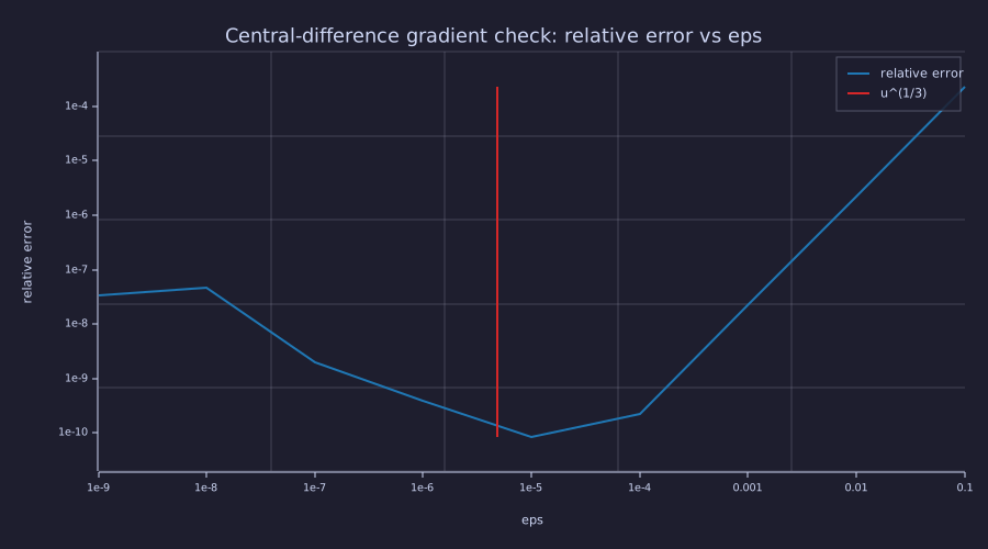
Read the V from the right: the clean descending branch (slope \(+2\), \(\varepsilon \ge 10^{-3}\)) is truncation error; the ragged ascending branch on the left (\(\varepsilon \le 10^{-6}\)) is cancellation error, growing roughly as \(1/\varepsilon\) and noisy because it is made of round-off; the red line is the predicted optimum \(u^{1/3}\).
The minimum lands at \(\varepsilon = 10^{-5}\) with relative error \(8.6e-11\), within a factor of two of the \(u^{1/3}\) prediction, and the right-hand branch has exactly the predicted slope (a factor of 100 per decade). Any \(\varepsilon\) between \(10^{-3}\) and \(10^{-7}\) would have passed the \(10^{-5}\) threshold; \(10^{-1}\) would not have.
Example — End-to-end training on the abb corpus
With the gradient verified, train for 600 AdamW steps with warmup+cosine. Each step is forward → upstream gradient → backward → AdamW, all from the library:
n_train = 600;  T_w = 60;  eta_max = 0.05;  eta_min = 0.005;
bet1 = 0.9;  bet2 = 0.999;  eps_a = 1e-8;
[M, V] = adamw_init(P);

loss_curve = zeros(n_train + 1);
[lo, L0, cache] = transformer_forward(ids, mask, P);
loss_curve(1) = L0;
for step = 1:n_train
  eta_t = warmup_cosine(step, n_train, T_w, eta_max, eta_min);
  [lo, L, cache] = transformer_forward(ids, mask, P);
  loss_curve(step + 1) = L;
  dl = ce_dlogits(ids, mask, lo, cache.total);
  G = transformer_backward(ids, dl, cache, P);
  [P, M, V] = adamw_step(P, G, M, V, eta_t, step, bet1, bet2, eps_a, 0.0);
end

L_bigram = (4 * 0.0 + 4 * (-log(4.0 / 7.0)) + 3 * (-log(3.0 / 7.0))) / 11;
print("Step 0   L =", loss_curve(1));
print("Final    L =", loss_curve(n_train + 1));
print("Bigram floor =", L_bigram);Step 0 L = 0.6262746329095578
Final L = 0.000000003918572521921996
Bigram floor = 0.4345778848093911The loss starts at \(0.6263\) nats/pair (random init over a 2-token vocabulary; \(\ln 2 = 0.693\) would be the uniform guess) and ends at \(3.92e-09\) — essentially zero, decisively below the bigram floor of \(0.4346\). The model has learned to use context beyond the current token. Convergence to the analytic minimum is a strong end-to-end sanity check on the whole training loop, but (as noted above) the final loss alone cannot separate attention from the fixed-PE-plus-FFN route on this small fixed corpus. The decisive evidence that the backward pass — and in particular backprop through attention — is correct remains the finite-difference gradient check above.
Example — Loss curve against the bigram floor
figure();
semilogy(0:n_train, loss_curve, "color", "blue", "label", "train loss")
hold("on")
hline(L_bigram, "red", "bigram floor")
hold("off")
title("Single-block transformer: end-to-end loss vs bigram floor (log scale)")
xlabel("step")
ylabel("L (nats / pair)")
legend("train loss", "bigram floor")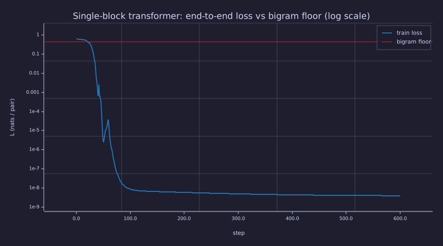
Three phases on the log axis: a transient over the first ~30 steps while \(\eta\) ramps, an exponential convergence (steps ~30–90) that crosses the bigram floor and drops seven decades, and a slow tail after step ~120 whose slope shrinks with the cosine-decayed learning rate — the loss is still seven orders of magnitude above the double-precision floor, so this is the schedule flattening, not round-off.
Example — Ablation: what actually beats the floor
Two mechanisms could carry the missing context-2 information: the attention head (reads earlier tokens) and the fixed positional code (every position is distinct, so the FFN can memorise a position→next-token table). Train four variants from the same snapshot P0, with the same seed, schedule and step count. Attention off clamps \(\mathbf{W}_O = \mathbf{0}\) after every update: then \(\mathbf{H}_{\text{mid}} = \mathbf{H}_{\text{in}} + \mathbf{O}\,\mathbf{0} = \mathbf{H}_{\text{in}}\) exactly, and piece (6) sends \(\bar{\mathbf{O}} = \overline{\mathrm{proj}}\,\mathbf{0} = \mathbf{0}\) into \(\bar{\mathbf{A}}, \bar{\mathbf{V}}, \bar{\mathbf{Q}}, \bar{\mathbf{K}}\) — the library trains the attention-free model without a second implementation. PE off zeroes the positional table.
function L_final = train_variant(P_start, ids, mask, n_steps, attn_on, T_w, eta_max, eta_min)
  Pv = P_start;
  d = size(Pv.E)(2);
  if attn_on == 0
    Pv.Wo = zeros(d, d);
  end
  [Mv, Vv] = adamw_init(Pv);
  for step = 1:n_steps
    eta_t = warmup_cosine(step, n_steps, T_w, eta_max, eta_min);
    [lo, L, ca] = transformer_forward(ids, mask, Pv);
    dlv = ce_dlogits(ids, mask, lo, ca.total);
    Gv = transformer_backward(ids, dlv, ca, Pv);
    [Pv, Mv, Vv] = adamw_step(Pv, Gv, Mv, Vv, eta_t, step, 0.9, 0.999, 1e-8, 0.0);
    if attn_on == 0
      Pv.Wo = zeros(d, d);
    end
  end
  [lo, L_final, ca] = transformer_forward(ids, mask, Pv);
end

P_nope = P0;  P_nope.PE = zeros(T_max, d_model);
L_abl = zeros(4);
L_abl(1) = train_variant(P0, ids, mask, n_train, 1, T_w, eta_max, eta_min);
L_abl(2) = train_variant(P0, ids, mask, n_train, 0, T_w, eta_max, eta_min);
L_abl(3) = train_variant(P_nope, ids, mask, n_train, 1, T_w, eta_max, eta_min);
L_abl(4) = train_variant(P_nope, ids, mask, n_train, 0, T_w, eta_max, eta_min);
print("full model               L =", L_abl(1));
print("attention off            L =", L_abl(2));
print("PE off                   L =", L_abl(3));
print("attention off and PE off L =", L_abl(4), " (bigram floor", L_bigram, ")");full model L = 0.000000003917458201133284
attention off L = 0.00000008155139693433182
PE off L = 0.4345792351431697
attention off and PE off L = 0.4345779208417609 (bigram floor 0.4345778848093911 )| Variant | Final loss (nats/pair) | Reaches the trigram floor 0? |
|---|---|---|
| full model | 3.92e-09 | yes |
| attention off (\(\mathbf{W}_O = 0\)) | 8.16e-08 | yes — position + FFN suffice |
| PE off | 0.4346 | no — sits on the bigram floor |
| attention off and PE off | 0.4346 | no — bigram floor \(0.4346\) |
On this corpus the honest reading is the opposite of the naive one: removing attention costs nothing (the FFN memorises a 12-entry position table), while removing the positional code alone drops the run onto the bigram floor — with identical token embeddings and no positions, the head can only form a bag-of-prefix average, and 600 steps do not turn that into a context-2 detector. Removing both reproduces the floor to four decimals. Beating a floor is evidence that some channel to the missing information exists, never evidence of which; the gradient check is what certifies attention's backward pass, and the ablation is what identifies the mechanism. The capstone repeats this table on a longer corpus, where both channels turn out to suffice alone.
Engineering Lenses
No signals reading adds to this lesson: the operators whose adjoints are derived here were read as filters, gain control and static nonlinearities in 08-scaled-dot-product-attention, 11-feed-forward-block and 12-layer-norm-and-residuals, and the backward pass adds no new signal.
Systems
Exact. The backward pass is one instance of the discrete-time adjoint (costate) recursion of 15-backpropagation. Read the block as a system stepped along depth, \(\mathbf{H}_{k+1} = \mathbf{H}_k + f_k(\mathbf{H}_k; \theta_k)\) with states \(\mathbf{H}_{\text{in}} \to \mathbf{H}_{\text{mid}} \to \mathbf{H}_{\text{out}}\) and a terminal cost \(\mathcal{L}(\mathbf{H}_{\text{out}})\). Then the costate is the adjoint of the state, \(\boldsymbol{\lambda}_k \equiv \bar{\mathbf{H}}_k\) (dH_out, dH_mid, dH_in in the code); the terminal condition is \(\boldsymbol{\lambda}_N = \partial\mathcal{L}/\partial\mathbf{H}_{\text{out}} = \bar{\mathbf{Z}}\mathbf{W}_U^\top\) (piece 2); the recursion is \(\boldsymbol{\lambda}_k = \boldsymbol{\lambda}_{k+1} + \left(\partial f_k/\partial \mathbf{H}_k\right)^{\!\top}\boldsymbol{\lambda}_{k+1}\) — the residual copy plus the branch's Jacobian-transpose product (pieces 3–7); and every parameter gradient is the Hamiltonian's derivative, \(\bar{\theta}_k = \sum_t \boldsymbol{\lambda}_{k+1}(t,:)^{\!\top}\,\partial f_k/\partial \theta_k\) — which is why each one has the form input' * upstream. Two consequences are checkable at once. The forward pass is nonlinear, but the adjoint system is linear in its terminal condition with coefficients frozen from the forward trajectory (cache): gradients scale and superpose. And the last-layer gradient is literally state-times-costate summed over time.
[lo, L_now, cache] = transformer_forward(ids, mask, P);
dl = ce_dlogits(ids, mask, lo, cache.total);
G  = transformer_backward(ids, dl, cache, P);
G2 = transformer_backward(ids, 2 * dl, cache, P);
seed(7);
dl_a = randn(T, vocab) * 0.1;  dl_b = randn(T, vocab) * 0.1;
Ga  = transformer_backward(ids, dl_a, cache, P);
Gb  = transformer_backward(ids, dl_b, cache, P);
Gab = transformer_backward(ids, dl_a + dl_b, cache, P);
lin_scale = max(max(abs(G2.Wq - 2 * G.Wq)));
lin_super = max(max(abs(Gab.E - Ga.E - Gb.E)));
H_out = cache.H_out;
costate_check = max(max(abs(G.W_U - H_out' * dl)));
print("scaling       max |G(2 dl) - 2 G(dl)|      =", lin_scale);
print("superposition max |G(a + b) - G(a) - G(b)| =", lin_super);
print("dW_U = H_out' * lambda_N max deviation =", costate_check);scaling max |G(2 dl) - 2 G(dl)| = 0
superposition max |G(a + b) - G(a) - G(b)| = 0.000000000000014210854715202004
dW_U = H_out' * lambda_N max deviation = 0Scaling holds exactly (deviation \(0\)) and superposition to \(1.4e-14\) (round-off): the backward pass is a linear time-varying system run in reverse depth, driven by the terminal costate. That linearity is what makes gradient accumulation over micro-batches, gradient clipping by rescaling, and the sum over positions in every input' * upstream legitimate.
Information
Exact. The bigram floor is not a property of any model; it is the conditional entropy of the corpus, \(H(\text{next} \mid \text{cur})\), and the trigram floor is \(H(\text{next} \mid \text{cur}, \text{prev})\). Their difference is the conditional mutual information \(I(\text{next}; \text{prev} \mid \text{cur})\) — the number of nats per pair that only a channel to the previous token can recover. Both are computed from (context, next) counts by cond_entropy_nats, a short helper defined in this notebook's hidden setup block on top of entropy_nats from lib/info.rlab:
H_cur      = cond_entropy_nats(ids, 1, vocab);
H_cur_prev = cond_entropy_nats(ids, 2, vocab);
print("H(next | cur)        =", H_cur, "nats   (bigram floor L_bigram =", L_bigram, ")");
print("H(next | cur, prev)  =", H_cur_prev, "nats");
print("I(next ; prev | cur) =", H_cur - H_cur_prev, "nats =", (H_cur - H_cur_prev) / log(2), "bits per pair");H(next | cur) = 0.4345778848093911 nats (bigram floor L_bigram = 0.4345778848093911 )
H(next | cur, prev) = 0 nats
I(next ; prev | cur) = 0.4345778848093911 nats = 0.6269633592945237 bits per pair\(H(\text{next} \mid \text{cur}) = 0.4346\) nats reproduces the hand-derived floor exactly, and \(H(\text{next} \mid \text{cur}, \text{prev}) = 0\): one token of extra context removes all the uncertainty, so \(I(\text{next}; \text{prev} \mid \text{cur}) = 0.627\) bits per pair is the entire budget. Attention is one mechanism that gives a position access to that information; on a fixed corpus the positional code is another (the ablation table). A model's final loss tells you how much of \(I\) it recovered, not through which channel.
Key Takeaways
- The chain rule from 15-backpropagation composes into a complete backward pass through one transformer block in seven pieces: cross-entropy → logits, LM head, residual splits, FFN with \(\mathrm{GELU}'\), LayerNorm, attention (softmax row, scaled dot product, no mask backward), Q/K/V projections and the embedding scatter-add. Lines 267–334 of
lib/transformer.rlabare those pieces in order. - A central finite-difference check verifies correctness at relative error \(\sim 10^{-10}\); its ε V-curve has a truncation branch (slope \(+2\)) and a cancellation branch (slope \(-1\)) with the optimum near \(u^{1/3}\). Always run one on a new backward implementation.
- On a context-2 corpus the trained block drives the loss below the bigram floor toward 0 — but the ablation shows the positional code, not attention, is what does it on this fixed 12-token corpus. Beating a floor identifies that information was recovered, not how.
- The backward pass is the adjoint recursion: linear in the terminal costate, and the bigram floor is \(H(\text{next} \mid \text{cur})\) of the corpus.
- The forward/backward pair, the AdamW step, and the schedule live once in
lib/transformer.rlab; the capstone and the fine-tuning lesson reuse them unchanged.
Standalone Scripts
| Script | What it computes |
|---|---|
full_backprop.rlab | Gradient check at \(W_U(1, 1)\) and \(W_q(1, 1)\); 600-step AdamW pretraining on the abb corpus; loss-curve figure. Pulls the forward/backward library in with run "../../lib/transformer.rlab". |
epsilon_vcurve.rlab | Sweeps \(\varepsilon \in \{10^{-1}, \dots, 10^{-9}\}\) in the central-difference check at \(W_U(1, 1)\) and saves the log–log V-curve. |
ablation_attention_pe.rlab | Trains the four variants (full / attention off / PE off / both off) from one initialisation and prints the final losses beside \(H(\text{next} \mid \text{cur})\) and \(H(\text{next} \mid \text{cur}, \text{prev})\) from lib/info.rlab. |
Run with make lesson-22 (or rustlab run lessons/22-full-backprop-through-the-block/<script>.rlab).
Expected Numerical Outputs Summary
| Variable | Expected Value |
|---|---|
rel_WU (gradient-check rel error, LM head) | \(\approx 2.2 \times 10^{-10}\) |
rel_q (gradient-check rel error, attention) | \(\approx 6.2 \times 10^{-11}\) |
eps_best (V-curve minimum) | \(10^{-5}\), rel error \(\approx 8.6 \times 10^{-11}\) |
loss_curve(1) (random init) | \(\approx 0.6263\) nats/pair |
L_bigram (bigram floor on abb) | \(0.4346\) nats/pair |
loss_curve(601) (after 600 steps) | \(\approx 3.9 \times 10^{-9}\) |
L_abl (full / attention off / PE off / both off) | \(\approx 3.9 \times 10^{-9}\) / \(8.2 \times 10^{-8}\) / \(0.4346\) / \(0.4346\) |
lin_scale, lin_super (adjoint linearity) | \(0\), \(\approx 1.4 \times 10^{-14}\) |
H_cur, H_cur_prev | \(0.4346\) nats, \(0\) nats |
Exercises
- Numerical-vs-analytical for every parameter. Extend the gradient check to
gamma1(1)(a LayerNorm scale). Why is the LayerNorm gradient harder to get right than the LM head's? - Why 0.434 is an entropy. Show by hand that the optimal bigram's cross-entropy on
abbabbabbabbequals \(H(\text{next} \mid \text{cur}) = \tfrac{7}{11}\,H\!\left(\tfrac{4}{7}, \tfrac{3}{7}\right)\) nats, and that any model conditioning only on the current token and carrying no position information cannot beat it.
Solution
The optimal bigram assigns the empirical conditional frequencies, \(P(\cdot \mid c) = n(c, \cdot)/n(c)\), so its mean cross-entropy is \(-\tfrac{1}{N}\sum_{t} \log P(x_{t+1} \mid x_t) = \sum_c \tfrac{n(c)}{N} \sum_{x} \tfrac{n(c,x)}{n(c)} \left(-\log \tfrac{n(c,x)}{n(c)}\right) = \sum_c \tfrac{n(c)}{N} H(\text{next} \mid \text{cur} = c)\), which is the definition of \(H(\text{next} \mid \text{cur})\). Here \(n(a) = 4\) with a deterministic successor (\(H = 0\)) and \(n(b) = 7\) with successors \(b, a\) in proportion \(4 : 3\), giving \(\tfrac{7}{11}\,H(\tfrac{4}{7}, \tfrac{3}{7}) = \tfrac{1}{11}\left(4 \log\tfrac{7}{4} + 3 \log\tfrac{7}{3}\right) = 0.4346\) nats. Any model whose output depends only on the current token is a bigram, and Gibbs' inequality bounds its cross-entropy below by that conditional entropy; position information breaks the premise because it makes the two b contexts distinguishable.
- Forward-difference V-curve. Repeat the ε sweep with the one-sided difference \((L(\theta + \varepsilon) - L(\theta))/\varepsilon\). Show that the truncation branch now has slope \(+1\) instead of \(+2\) and that the optimum moves from \(u^{1/3}\) to \(u^{1/2} \approx 1.05 \times 10^{-8}\) (with \(u = 2^{-53} \approx 1.1 \times 10^{-16}\)).
- Trainable positional embedding. Derive \(\bar{\mathbf{PE}}\) and write the lines you would add to
transformer_backwardandadamw_stepto train it.
Solution
\(\mathbf{H}_{\text{in}} = \mathbf{X}_{\text{1-hot}}\mathbf{E} + \mathbf{PE}(1{:}T, :)\), so the adjoint of the sum is copied: \(\bar{\mathbf{PE}}(t,:) = \bar{\mathbf{H}}_{\text{in}}(t,:)\) for \(t \le T\) and \(\mathbf{0}\) for the unused rows \(t > T\) — an identity "scatter" because each position is used exactly once. In code: dPE = zeros(T_max, d_model); dPE(1:T, :) = dH_in; added to G as field PE, and one more adamw_update line for P.PE in adamw_step.
- Multi-head. With \(h\) heads of width \(d_k = d/h\) (09-multi-head-attention), which of the seven pieces change and which lines of
mha_block_forwardwould need a backward pass? (Only piece 6: per-head \(\mathbf{A}_h, \mathbf{V}_h, \mathbf{Q}_h, \mathbf{K}_h\) with the \(1/\sqrt{d_k}\) scale, and the concatenation becomes a column-slice scatter into \(\bar{\mathbf{Q}}, \bar{\mathbf{K}}, \bar{\mathbf{V}}\).)
What's next
23-putting-it-all-together is the capstone: the same library trains a single-block transformer on a BPE-tokenised corpus, checkpoints it, generates text under every sampling strategy, and repeats this lesson's ablation — every component of the curriculum in one run. 25-fine-tuning-sft-and-dpo then reuses the backward pass for supervised fine-tuning and direct preference optimisation.