Lesson 03: Cross-Entropy Loss
The model outputs a probability distribution. The ground truth is the actual next token. We need a scalar that measures how wrong the prediction is — this scalar is the cross-entropy loss, and minimising it is the entire goal of training. Its gradient with respect to the logits, \(\hat{\mathbf{p}} - \mathbf{y}\), is the error signal that every later lesson feeds back into the parameters.
Learning Objectives
- Define cross-entropy between a true distribution and a predicted distribution, in nats and in bits.
- Derive the simplified cross-entropy loss used in language model training and its maximum-likelihood origin step by step.
- Derive the gradient with respect to the logits, \(\partial \mathcal{L} / \partial \mathbf{z} = \hat{\mathbf{p}} - \mathbf{y}\), and explain why it is bounded even when the prediction is catastrophically wrong.
- Read the loss surface in logit space: the asymptotic floor, the linear wall, and its convexity.
- Compute cross-entropy, a KL divergence, and the Gaussian-likelihood form of MSE by hand and verify against the simulation output.
Background
Probability distributions, softmax, entropy, and the log-sum-exp from 02-probability-and-softmax; one-hot vectors from 01-tokens-and-encoding; the notation of 00-the-llm-as-a-system (losses in nats in code, bits in prose). Natural logarithm \(\ln(x) = \log_e(x)\). The concept of a loss function: a scalar that measures how wrong a model's prediction is.
The Setup
At each position in a sequence the model outputs \(\hat{\mathbf{p}} \in \mathbb{R}^{|\mathcal{V}|}\) (a probability distribution from softmax, 02-probability-and-softmax). The ground truth is the actual next token — a one-hot vector \(\mathbf{y}\) (01-tokens-and-encoding).
Cross-Entropy
Theory
The cross-entropy between the true distribution \(\mathbf{y}\) and predicted distribution \(\hat{\mathbf{p}}\) is
\[H(\mathbf{y}, \hat{\mathbf{p}}) = -\sum_{i=1}^{|\mathcal{V}|} y_i \log \hat{p}_i.\]
Because \(\mathbf{y}\) is one-hot, only the term for the correct token \(c\) survives:
\[\mathcal{L} = -\log \hat{p}_c.\]
This is the negative log-probability of the correct token — the standard loss for language model training. With the natural logarithm the unit is the nat; dividing by \(\ln 2\) gives bits (the course convention: nats in code, bits in prose). Reference values:
| \(\hat{p}_c\) | \(\mathcal{L}\) (nats) | \(\mathcal{L}\) (bits) | Meaning |
|---|---|---|---|
| 1.0 | 0 | 0 | Perfect prediction |
| 0.5 | 0.693 | 1 | A fair coin's worth of doubt |
| 0.25 | 1.386 | 2 | Uniform over four tokens |
| 0.01 | 4.605 | 6.64 | Nearly zero probability on the right answer |
| \(\to 0\) | \(\to \infty\) | \(\to \infty\) | Catastrophically wrong |
As a function of \(\hat{p}_c\) the loss is convex and decreasing; the unbounded tail as \(\hat{p}_c \to 0\) is why a single confidently wrong token can dominate a batch.
Example — Loss curve and reference points
% Sample p_hat across (0.01, 1.0] and compute L = -log(p_hat_c) in nats
p_hat = linspace(0.01, 1.0, 200);
loss = -log(p_hat);L_50k = -log(1.0 / 50000.0);
L_4 = -log(0.25);
L_half = -log(0.5);
L_high = -log(0.9);
L_vhigh = -log(0.99);
print("nats:", L_50k, L_4, L_half, L_high, L_vhigh);
print("bits:", L_50k / log(2), L_4 / log(2), L_half / log(2), L_high / log(2), L_vhigh / log(2));nats: 10.819778284410283 1.3862943611198906 0.6931471805599453 0.10536051565782628 0.01005033585350145
bits: 15.609640474436812 2 1 0.15200309344504997 0.01449956969511509Reference points in nats: \(p{=}1/50000 \Rightarrow L = 10.820\) (the uniform-over-50k-tokens baseline, \(15.61\) bits), \(p{=}0.25 \Rightarrow L = 1.386\) (\(= \log 4\), exactly 2 bits), \(p{=}0.5 \Rightarrow L = 0.693\) (1 bit), \(p{=}0.9 \Rightarrow L = 0.105\), \(p{=}0.99 \Rightarrow L = 0.0101\).
figure();
hold("on")
plot(p_hat, loss, "color", "blue", "label", "L = -log(p)")
hline(L_4, "gray", "baseline = log(4)")
title("Cross-Entropy Loss vs. Predicted Probability of Correct Token")
xlabel("Predicted probability of correct token (p_c)")
ylabel("Loss L = -log(p_c)  [nats]")
ylim([0, 6])
legend()
hold("off")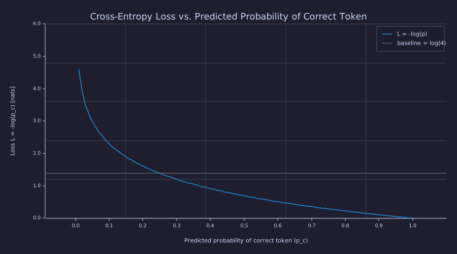
The curve crosses the grey baseline at \(\hat{p}_c = 0.25\): any prediction to the left of that point is worse than guessing on a four-token vocabulary. The steepening toward \(\hat{p}_c \to 0\) is the unbounded penalty for confident errors.
At \(\hat{p}_c = 1/|\mathcal{V}|\) (uniform prediction — the model knows nothing), the loss equals \(\log |\mathcal{V}|\). This is the baseline loss at the start of training.
Connection to Maximum Likelihood
Theory
A language model assigns a probability to a whole training sequence \(x_1, \dots, x_T\) by the chain rule of probability, one factor per position:
\[P_\theta(x_1, \dots, x_T) = \prod_{t=1}^{T} \hat{p}^{(t)}_{x_t}, \qquad \hat{p}^{(t)} = \text{the model's distribution at position } t \text{ given } x_{<t}.\]
Maximum likelihood chooses the parameters \(\theta\) that make the observed corpus most probable. Four steps turn that into the loss above:
- Product → log. The logarithm is monotone, so maximising \(P_\theta\) and maximising \(\log P_\theta\) pick the same \(\theta\), and the product becomes a sum: \(\log P_\theta = \sum_{t=1}^{T} \log \hat{p}^{(t)}_{x_t}\).
- Maximise → minimise. Negate: minimising \(-\log P_\theta = \sum_t \bigl(-\log \hat{p}^{(t)}_{x_t}\bigr)\) — each term is one token's cross-entropy \(\mathcal{L}_t\).
- Sum → mean. Divide by \(T\) so the number does not grow with corpus length: \[\mathcal{L}_{\text{avg}} = -\frac{1}{T} \sum_{t=1}^{T} \log \hat{p}^{(t)}_{x_t}.\]
- Read the units. \(\mathcal{L}_{\text{avg}}\) is the average negative log-likelihood per token — nats per token, or bits per token after \(\div \ln 2\).
Minimising cross-entropy is maximum likelihood estimation; nothing was added or dropped along the way. For probabilities \([0.7, 0.4, 0.9]\) on three correct tokens the product is \(0.252\) and \(-\ln(\cdot)/3\) gives the mean loss \(0.4594\) nats — the same information, on a per-token scale.
Gradient of the Loss
Theory
Real models never touch \(\hat{p}_c\) directly: they produce logits \(\mathbf{z}\) and softmax turns them into \(\hat{\mathbf{p}}\) (02-probability-and-softmax). The derivative the optimiser actually sees is therefore \(\partial \mathcal{L} / \partial \mathbf{z}\), and it is best derived from the loss written in terms of logits. Using \(\hat{p}_c = e^{z_c} / \sum_j e^{z_j}\),
\[\mathcal{L} = -\log \hat{p}_c = -z_c + \log \sum_{j} e^{z_j} = -z_c + \mathrm{LSE}(\mathbf{z}),\]
where \(\mathrm{LSE}\) is the log-sum-exp — the log of the partition function \(Z\) from Lesson 02. Its gradient is the softmax itself: \(\partial\, \mathrm{LSE} / \partial z_j = e^{z_j} / \sum_k e^{z_k} = \hat{p}_j\). Differentiating both terms,
\[\frac{\partial \mathcal{L}}{\partial z_j} = -\mathbf{1}[j = c] + \hat{p}_j, \qquad\text{i.e.}\qquad \boxed{\frac{\partial \mathcal{L}}{\partial \mathbf{z}} = \hat{\mathbf{p}} - \mathbf{y}.}\]
Three facts follow, and the third is the one to remember:
- It is the prediction error. Each component is (predicted mass) − (target mass): negative on the correct class (push \(z_c\) up), positive on every other class (push it down).
- It sums to zero, because both \(\hat{\mathbf{p}}\) and \(\mathbf{y}\) sum to one. Adding a constant to all logits cannot change the loss, so the gradient has no component along the all-ones direction.
- It is bounded. Every component lies in \([-1, 1]\) and \(\lVert \hat{\mathbf{p}} - \mathbf{y} \rVert_1 \le 2\), no matter how wrong the model is. Contrast \(d\mathcal{L}/d\hat{p}_c = -1/\hat{p}_c\), which is \(-100\) at \(\hat{p}_c = 0.01\): that quantity exists, but the optimiser never sees it, because the softmax Jacobian multiplies it by \(\hat{p}_c(1 - \hat{p}_c)\) on the way back to the logits. A confidently wrong prediction produces a large loss, not a large gradient — the signal saturates at \(\pm 1\).
The loss is also convex in \(\mathbf{z}\): \(-z_c\) is linear, and \(\mathrm{LSE}\) has Hessian \(\mathrm{diag}(\hat{\mathbf{p}}) - \hat{\mathbf{p}}^\top \hat{\mathbf{p}}\), which is positive semi-definite (it is the covariance matrix of a one-hot draw from \(\hat{\mathbf{p}}\)). Every non-convexity in language-model training is introduced by the network that produces \(\mathbf{z}\) (06-linear-layers-and-gradient-descent onward), never by the loss.
Example — The error signal for a three-class prediction
z3 = [1.0, 2.0, 0.0];             % logits: the distractor (class 2) currently wins
c3 = 1;                           % correct class
p3 = softmax(z3);
y3 = zeros(3); y3(c3) = 1.0;
g3 = p3 - y3;                     % dL/dz
L3 = -z3(c3) + log(sum(exp(z3))); % the LSE form of the loss
print("p_hat      =", p3);
print("dL/dz      =", g3);
print("sum(dL/dz) =", sum(g3), "   max|dL/dz| =", max(abs(g3)));
print("L via LSE =", L3, " -log p_c =", -log(p3(c3)));p_hat = [1×3] 0.244728 0.665241 0.090031
dL/dz = [1×3] -0.755272 0.665241 0.090031
sum(dL/dz) = -0.00000000000000008326672684688674 max|dL/dz| = 0.7552715289452023
L via LSE = 1.4076059644443801 -log p_c = 1.4076059644443804With \(\hat{p}_c = 0.245\) the loss is \(1.408\) nats, yet the largest gradient component is only \(0.755\) — and it would stay below 1 even at \(\hat{p}_c = 10^{-6}\). The optimiser's signal is the error vector, not the loss's slope in \(\hat{p}\).
The Loss Surface in Logit Space
Theory
For a 3-class problem with logits \(\mathbf{z} = (z_1, z_2, z_3{=}0)\) and the correct class \(c = 1\):
\[\hat{p}_1 = \frac{e^{z_1}}{e^{z_1} + e^{z_2} + 1}, \qquad \mathcal{L}(z_1, z_2) = -z_1 + \log\!\left(e^{z_1} + e^{z_2} + 1\right).\]
That is a 2-parameter surface — the canonical "loss bowl" gradient descent actually sees, and (by the Hessian argument above) a convex one.
Example — 2-D loss surface over \((z_1, z_2)\)
n = 60;
z1_grid = linspace(-3.0, 5.0, n);
z2_grid = linspace(-3.0, 5.0, n);
[Z1, Z2] = meshgrid(z1_grid, z2_grid);

L_surface = -Z1 + log(exp(Z1) + exp(Z2) + 1.0);
L_flat = reshape(L_surface, 1, n * n);
L_min = min(L_flat);
L_max = max(L_flat);
print("L_surface on the grid: min =", L_min, " max =", L_max);L_surface on the grid: min = 0.00704851041106469 max = 8.007048510411064Range on the grid: loss spans \([0.007, 8.007]\) nats — near-zero when \(z_1\) dominates, linearly large when the distractor \(z_2\) wins.
figure();
contourf(Z1, Z2, L_surface, 20)
title("CE loss over logit space (z3 = 0, correct = class 1)")
xlabel("z1 (correct)")
ylabel("z2 (distractor)")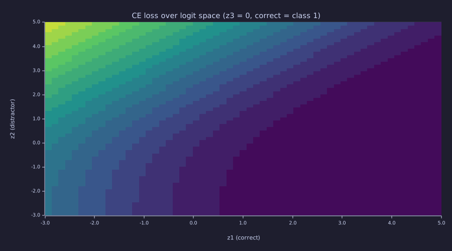
Toward the upper-left (distractor winning) the filled bands are evenly spaced parallel stripes: the loss climbs linearly with \(z_2 - z_1\). Toward the lower-right the bands stop — the loss flattens onto its floor near zero without ever reaching it.
Three features of this surface make the training dynamics legible:
- Asymptotic floor. Push \(z_1\) to infinity and the loss approaches 0 — but never reaches it. There is no finite minimiser, which is why LM training never converges to "zero loss" on a finite dataset without overfitting.
- Linear wall in the distractor direction. When \(z_2 \gg z_1\) the loss grows like \(z_2 - z_1\) — a linear ramp, not an exponential cliff. Its slope is the bounded gradient of the previous section: \(\partial \mathcal{L}/\partial z_2 = \hat{p}_2 \to 1\).
- Convex, no local minima. Every contour is a convex curve, so from any starting logits the negative gradient points into the same basin.
Sidebar: Label Smoothing
Theory
The cross-entropy target so far is a hard one-hot vector: \(y_i = 1\) for the correct class, 0 elsewhere. Label smoothing softens that target by reserving a small mass \(\varepsilon\) (typically 0.1) for the rest of the vocabulary:
\[y^{\text{smooth}}_i = (1 - \varepsilon)\,\mathbf{1}_{i = c} + \frac{\varepsilon}{|\mathcal{V}|}.\]
The loss against the smoothed target is
\[\mathcal{L}_{\text{smooth}} = -\sum_i y^{\text{smooth}}_i \log \hat p_i = (1 - \varepsilon)\bigl(-\log \hat p_c\bigr) + \varepsilon \, H(\mathbf{u}, \hat{\mathbf{p}}), \qquad H(\mathbf{u}, \hat{\mathbf{p}}) = -\frac{1}{|\mathcal{V}|}\sum_i \log \hat p_i,\]
where the second term is the cross-entropy of \(\hat{\mathbf{p}}\) against the uniform distribution \(\mathbf{u}\). The net effect: the optimum at \(\hat p_c = 1\) becomes \(\hat p_c = 1 - \varepsilon + \varepsilon/|\mathcal{V}|\) — the model is forbidden from putting all its mass on the correct class.
Why it helps
- Calibration. Without smoothing, well-trained models become overconfident — they assign 0.999+ to whichever token they pick, even on inputs where they should be uncertain. Smoothing keeps probabilities calibrated.
- Generalisation. The smoothed target acts as a mild regulariser; it discourages extreme logits and reduces overfitting on small datasets.
- Beam search compatibility. The original Attention Is All You Need paper trained with \(\varepsilon = 0.1\) and reported only that it hurt perplexity while improving accuracy and BLEU. A common interpretation is that smoothing helps beam search explore — an overconfident model whose top token sits at 0.999-vs-0.001 lets a single hypothesis dominate the beam score — but the paper does not state this as its reason.
Modern GPT-style models (including nanoGPT) do not use label smoothing — open-ended text generation cares about ranking, not calibration, and large-scale training has its own regularisation effects (data scale, dropout, weight decay). It is still standard in machine translation and any task where calibrated probabilities matter.
Engineering Lenses
The loss is where the information view and the systems view of training first meet: it is a code length, and its gradient is an error signal. No signals-and-filters reading adds to this lesson (log-sum-exp is a smooth maximum, and that is the whole of it), so that lens is omitted.
Systems
Exact. \(\partial \mathcal{L} / \partial \mathbf{z} = \hat{\mathbf{p}} - \mathbf{y}\) is the only quantity the loss hands to the rest of the training machinery. Every gradient in the network (15-backpropagation) is this vector multiplied by Jacobians, and every parameter update (06-linear-layers-and-gradient-descent, 16-adamw-optimizer) is a filtered, scaled version of it.
Model. Read as a control loop, \(\mathbf{y}\) is the set point, \(\hat{\mathbf{p}}\) the measured output, and \(\hat{\mathbf{p}} - \mathbf{y}\) the error — a bounded error, because softmax + cross-entropy act as a soft-decision detector whose error saturates at \(\pm 1\). The forward path and the backward path form the pair drawn below; Lessons 06 and 15–18 close the loop around it.
The saturation is easiest to see in the two-alternative case. Hold the distractor logits fixed at \(m = \mathrm{LSE}(\mathbf{z}_{\ne c})\) and sweep \(z_c\): then \(\hat{p}_c = \sigma(z_c - m)\), the logistic sigmoid of the logit margin, and \(\partial \mathcal{L}/\partial z_c = \hat{p}_c - 1\).
margin = linspace(-6.0, 6.0, 121);        % z_c - LSE(other logits)
p_c    = 1.0 ./ (1.0 + exp(-margin));      % forward: p_hat_c as a function of the margin
g_c    = p_c - 1.0;                        % backward: dL/dz_c
L_c    = -log(p_c);                        % the loss itself, for contrast
print("margin -6: loss =", L_c(1), "nats   dL/dz_c =", g_c(1));

figure();
hold("on")
plot(margin, L_c, "color", "green", "label", "L = -log p_c  (loss)")
plot(margin, p_c, "color", "blue", "label", "p_c  (forward)")
plot(margin, g_c, "color", "red", "label", "dL/dz_c = p_c - 1  (backward)")
hline(-1.0, "gray", "saturation at -1")
title("Loss, forward probability and backward error signal vs. logit margin")
xlabel("logit margin  z_c - LSE(others)")
ylabel("value")
legend()
hold("off")margin -6: loss = 6.00247568513773 nats dL/dz_c = -0.9975273768433652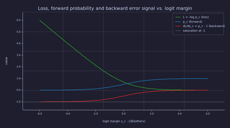
The red error signal is a shifted sigmoid that flattens onto the grey rail at \(-1\) for large negative margins, while the green loss over the same margins keeps climbing linearly. Being very wrong costs loss without buying a larger gradient.
At a margin of \(-6\) the loss is \(6.00\) nats but the gradient is \(-0.9975\) — already at the rail.
Information
Exact. Cross-entropy decomposes as
\[H(\mathbf{p}, \hat{\mathbf{p}}) = H(\mathbf{p}) + D_{\text{KL}}(\mathbf{p} \,\|\, \hat{\mathbf{p}}),\]
where \(H(\mathbf{p})\) is the entropy of the true distribution and \(D_{\text{KL}} \ge 0\) is the Kullback–Leibler divergence. For a one-hot \(\mathbf{y}\), \(H(\mathbf{y}) = 0\), so the per-token loss is the KL divergence from the target. In coding terms (02-probability-and-softmax): the optimal code for symbol \(i\) under \(\mathbf{p}\) has length \(-\log_2 p_i\) bits; if the source is \(\mathbf{p}\) but the code is built from the model's \(\hat{\mathbf{p}}\), the expected length is \(\mathbb{E}_{i \sim \mathbf{p}}[-\log_2 \hat p_i] = H(\mathbf{p}, \hat{\mathbf{p}})\), and the KL term is exactly the excess bits the mismatch costs. Computed on Lesson 02's logits, with the \(\tau = 1\) softmax as the source and the flatter \(\tau = 2\) softmax as the model:
z02   = [2.0, 1.0, 0.5, -0.5];       % Lesson 02's logits
p_src = softmax(z02 / 1.0);           % "true" source: tau = 1
p_mdl = softmax(z02 / 2.0);           % the model's code: tau = 2
H_src  = entropy_bits(p_src);
H_x    = cross_entropy_bits(p_src, p_mdl);
KL_sm  = kl_bits(p_src, p_mdl);
KL_rev = kl_bits(p_mdl, p_src);
print("H(p)         =", H_src, "bits");
print("H(p, p_hat)  =", H_x, "bits");
print("KL(p||p_hat) =", KL_sm, "bits   (excess bits per symbol)");
print("KL(p_hat||p) =", KL_rev, "bits (not symmetric)");H(p) = 1.525296073088579 bits
H(p, p_hat) = 1.6334739224072374 bits
KL(p||p_hat) = 0.10817784931865848 bits (excess bits per symbol)
KL(p_hat||p) = 0.11990712442392848 bits (not symmetric)Coding this source with the \(\tau = 2\) code costs \(1.633\) bits per symbol instead of the \(1.525\)-bit optimum — an overhead of \(0.108\) bits, \(7.1\) %. Reversing the roles gives \(0.120\) bits: KL is a divergence, not a distance.
Exact. Mean squared error is cross-entropy under a Gaussian noise model. If a regression model predicts \(\hat y\) and the observation is \(y = \hat y + \text{noise}\) with \(\mathcal{N}(0, \sigma^2)\) noise, then
\[-\log \mathcal{N}(y;\, \hat y, \sigma^2) = \frac{(y - \hat y)^2}{2\sigma^2} + \tfrac{1}{2}\log(2\pi\sigma^2),\]
the squared error plus a constant. The MSE that 06-linear-layers-and-gradient-descent minimises is therefore the same objective as this lesson's — maximum likelihood — under a different noise model: Gaussian on a real value instead of categorical on a token.
y_obs = 2.0;  y_pred = [0.0, 1.0, 2.0, 3.0, 4.0];  sigma = 1.0;
nll_gauss = 0.5 * log(2 * pi * sigma^2) + (y_obs - y_pred) .^ 2 / (2 * sigma^2);
half_sq   = (y_obs - y_pred) .^ 2 / 2;
print("Gaussian NLL      :", nll_gauss);
print("NLL - (y-y_hat)^2/2:", nll_gauss - half_sq);Gaussian NLL : [1×5] 2.918939 1.418939 0.918939 1.418939 2.918939
NLL - (y-y_hat)^2/2: [1×5] 0.918939 0.918939 0.918939 0.918939 0.918939The difference is the constant \(\tfrac{1}{2}\log 2\pi = 0.9189\) at every prediction — it shifts the loss but not its gradient, so minimising Gaussian NLL and minimising squared error select the same parameters.
Model. Maximum likelihood is minimum description length — for a fixed model class, since ML minimises only the data term of the description length, not the cost of the model itself. Minimising \(-\sum_t \log_2 \hat p_{x_t}\) minimises the number of bits needed to transmit the corpus under the model, so a better language model is a better compressor of its training distribution; the mechanism (arithmetic coding) and the bits-per-character bookkeeping are in 20-perplexity-and-evaluation. Modern reporting uses bits per byte or bits per character; Shannon's own experiments put English at roughly 0.6–1.3 bits per character,1 and the best current models sit near the low end of that range. 05-bigram-language-model introduces perplexity \(= e^{\mathcal{L}_{\text{nats}}} = 2^{\mathcal{L}_{\text{bits}}}\) — the same bound read as an effective alphabet size.
C. E. Shannon, "Prediction and Entropy of Printed English", Bell System Technical Journal 30(1), 1951.
Key Takeaways
- Cross-entropy loss \(\mathcal{L} = -\log \hat{p}_c\) is the standard training objective for language models: nats in code, bits (\(\div \ln 2\)) in prose.
- Its gradient with respect to the logits is \(\hat{\mathbf{p}} - \mathbf{y}\): a bounded, zero-sum error signal. The loss is unbounded as \(\hat{p}_c \to 0\); the gradient is not.
- Cross-entropy \(\neq\) accuracy. A model that assigns \(\hat{p}_c = 0.51\) to the correct token at every position wins the \(\arg\max\) every time — 100% accuracy — yet still carries a loss of \(-\ln 0.51 \approx 0.67\) nats. Loss measures confidence in the correct token; accuracy measures only whether it tops the \(\arg\max\).
- Training a language model is maximum likelihood estimation; MSE is the same principle under Gaussian noise. The loss is convex in the logits — non-convexity enters with the network.
Standalone Scripts
| Script | What it computes |
|---|---|
cross_entropy_surface.rlab | \(\mathcal{L}(\hat{p}_c) = -\log\hat{p}_c\) as a 1-D curve; the logit gradient \(\hat{\mathbf{p}} - \mathbf{y}\) for the 3-class example; the 2-D loss surface over \((z_1, z_2)\) as filled contours |
ce_gradient_and_kl.rlab | the saturating error signal vs. logit margin; the KL divergence between Lesson 02's \(\tau = 1\) and \(\tau = 2\) softmaxes; the Gaussian-NLL ⇔ MSE identity |
Run with make lesson-03 (or rustlab run lessons/03-cross-entropy-loss/<name>.rlab).
Expected Numerical Outputs Summary
| Variable | Expected Value |
|---|---|
L_50k (\(-\log(1/50000)\)) | ≈ 10.820 nats (15.61 bits) |
L_4 (\(-\log 0.25\)) | ≈ 1.386 nats (2 bits) |
L_half (\(-\log 0.5\)) | ≈ 0.693 nats (1 bit) |
L_high (\(-\log 0.9\)) | ≈ 0.105 nats |
L_vhigh (\(-\log 0.99\)) | ≈ 0.0101 nats |
p3 for \(\mathbf{z} = (1, 2, 0)\) | ≈ [0.245, 0.665, 0.090] |
g3 \(= \hat{\mathbf{p}} - \mathbf{y}\) | ≈ [-0.755, 0.665, 0.090]; sums to 0 |
L_surface minimum | ≈ 0.007 nats (corner where \(z_1\) dominates) |
L_surface maximum | ≈ 8.007 nats (corner where \(z_2\) dominates) |
H_src, H_x | ≈ 1.525, 1.633 bits |
KL_sm, KL_rev | ≈ 0.108, 0.120 bits |
nll_gauss - half_sq | 0.9189 (= \(\tfrac{1}{2}\log 2\pi\)) everywhere |
Exercises
-
Baseline loss. At the start of training, a model outputs a uniform distribution over a vocabulary of size 50,000. What is the cross-entropy loss? Express this as \(\ln(|\mathcal{V}|)\) and compute the numerical value in nats and in bits.
-
Loss ceiling. If a model assigns probability \(10^{-6}\) to the correct token, what is the cross-entropy loss? Is this worse or better than a uniform prediction over a 50-token vocabulary? What is the gradient \(\partial \mathcal{L}/\partial z_c\) in that case?
-
Sequence loss. A model processes a 3-token sequence and assigns probabilities \([0.8, 0.3, 0.6]\) to the correct tokens. Compute the mean cross-entropy loss \(\mathcal{L}_{\text{avg}}\).
-
Where the \(1/\hat{p}_c\) goes. Starting from \(d\mathcal{L}/d\hat{p}_c = -1/\hat{p}_c\) and the softmax Jacobian \(\partial \hat{p}_c / \partial z_j = \hat{p}_c(\mathbf{1}[j = c] - \hat{p}_j)\), apply the chain rule and show that \(\partial \mathcal{L}/\partial z_j = \hat{p}_j - \mathbf{1}[j = c]\). At which step does the unbounded factor cancel?
Solution
\(\partial \mathcal{L}/\partial z_j = (d\mathcal{L}/d\hat{p}_c)(\partial \hat{p}_c/\partial z_j) = -\tfrac{1}{\hat{p}_c}\cdot \hat{p}_c(\mathbf{1}[j = c] - \hat{p}_j) = \hat{p}_j - \mathbf{1}[j = c]\). The \(\hat{p}_c\) in the Jacobian cancels the \(1/\hat{p}_c\) from the log immediately — the unbounded factor never survives to the logits.
-
Loss curve units. Modify
cross_entropy_surface.rlabto plot \(-\log_2(\hat{p}_c)\) instead of natural log. How does the shape change? What is the unit of the resulting loss? At what probability does the loss equal 1 bit?
What's next
04-embeddings-and-similarity replaces the orthogonal one-hot vectors of Lesson 01 with dense embedding vectors that carry geometric meaning. The loss function from this lesson stays — the only change is what the model sees as input. The error signal \(\hat{\mathbf{p}} - \mathbf{y}\) returns in 06-linear-layers-and-gradient-descent (as the gradient of the bigram model written as a linear layer) and in 15-backpropagation (as the start of every backward pass).