Lesson 05: The Bigram Language Model
A language model assigns a probability to every possible next token. The bigram model makes the simplest possible assumption: the next token depends only on the current one. Despite its simplicity, it introduces the full train-then-sample loop that every neural language model follows — and it is the first component of the course that is exactly a dynamical system, a Markov chain, so the Systems lens at the end of this lesson is an identity rather than an analogy.
Learning Objectives
- Define a bigram language model and derive its count-based estimator as the maximum-likelihood solution.
- Construct a bigram count matrix from a corpus and normalise it into a row-stochastic probability matrix in one line.
- Trace inverse-transform sampling step by step, generate a sequence, and decode it back to text.
- Relate the row entropies of \(\mathbf{P}\) to the corpus cross-entropy through \(H(X_{t+1} \mid X_t) = \sum_i \pi_i H(\mathbf{P}_{i,:})\).
- Read \(\mathbf{P}\) as a discrete-time linear system: stationary distribution, eigenvalues on the unit circle, and why smoothing makes the chain mix.
Background
Tokens and vocabulary from 01-tokens-and-encoding. Probability distributions, entropy, and the max-entropy Lagrangian from 02-probability-and-softmax. Cross-entropy loss from 03-cross-entropy-loss (used to define the training objective; not strictly required to follow the count-based estimator).
The Language Modelling Problem
The goal is to estimate
\[P(x_{t+1} \mid x_1, x_2, \ldots, x_t).\]
The full history can be arbitrarily long. The bigram model makes the Markov assumption:
\[P(x_{t+1} \mid x_1, \ldots, x_t) \approx P(x_{t+1} \mid x_t).\]
This reduces the problem to estimating \(|\mathcal{V}|^2\) conditional probabilities — one for every ordered pair of tokens — arranged as a matrix \(\mathbf{P}\) with \(P_{ij} = P(x_{t+1} = j \mid x_t = i)\). Because every row is a probability distribution, \(\mathbf{P}\) is row-stochastic: \(P_{ij} \ge 0\) and \(\sum_j P_{ij} = 1\) for every \(i\). This is exactly the first-order Markov source of Shannon's 1948 paper (A Mathematical Theory of Communication, §3), where "artificial English" is generated by drawing each letter from the distribution conditioned on the previous one.
Building the Bigram Matrix
Theory
Step 1 — Count. Scan the corpus and tally every consecutive pair \((x_t, x_{t+1})\) into the count matrix \(\mathbf{C} \in \mathbb{Z}_{\geq 0}^{|\mathcal{V}| \times |\mathcal{V}|}\):
\[C_{ij} = \text{number of times token } j \text{ follows token } i.\]
Step 2 — Normalise. Divide each row by its sum:
\[P_{ij} = \frac{C_{ij}}{\sum_{k=1}^{|\mathcal{V}|} C_{ik}}.\]
In code that is one line — P = C ./ sum(C, 2) — the column vector of row sums broadcasts across the columns. We work the corpus "abcbabcba" end-to-end below.
Example — Counting bigrams in "abcbabcba"
% Corpus: "abcbabcba" — vocabulary a=1, b=2, c=3
vocab_size = 3;
seq    = [1, 2, 3, 2, 1, 2, 3, 2, 1];
tokens = {"a", "b", "c"};
n_tokens  = len(seq);
n_bigrams = n_tokens - 1;

% Build the count matrix
C = zeros(vocab_size, vocab_size);
for t = 1:n_bigrams
  C(seq(t), seq(t + 1)) = C(seq(t), seq(t + 1)) + 1;
end

print("Bigram count matrix C  (row=current, col=next):");
print(C);Bigram count matrix C (row=current, col=next):
Matrix(3x3)
[0.000000, 2.000000, 0.000000]
[2.000000, 0.000000, 2.000000]
[0.000000, 2.000000, 0.000000]The corpus has 9 tokens, producing 8 bigrams. Total counts sum to 8 — matches \(n_{\text{bigrams}}\).
Example — Row-normalising counts to probabilities
P = C ./ sum(C, 2);            % one line: each row divided by its own sum
print("Row-stochastic probability matrix P:");
print(P);
print("Row sums (each should be 1):", sum(P, 2)');Row-stochastic probability matrix P:
Matrix(3x3)
[0.000000, 1.000000, 0.000000]
[0.500000, 0.000000, 0.500000]
[0.000000, 1.000000, 0.000000]
Row sums (each should be 1): Matrix(1x3)
[1.000000, 1.000000, 1.000000]Token a always goes to b. Token c always goes to b. Token b goes to either a or c with equal probability. Drawn as a state graph, \(\mathbf{P}\) is a signal-flow diagram whose edge weights are the transition probabilities:
Every path through the graph alternates between \(\{a, c\}\) and \(\{b\}\) — keep that in mind for the Systems lens.
Laplace Smoothing
Theory
If a pair never appeared, \(P_{ij} = 0\) and the cross-entropy loss is infinite on that bigram. Add-one smoothing ensures every pair has non-zero probability:
\[P_{ij}^{\text{smooth}} = \frac{C_{ij} + 1}{\sum_k (C_{ik} + 1)} = \frac{C_{ij} + 1}{\sum_k C_{ik} + |\mathcal{V}|}.\]
(Add-\(k\) smoothing replaces the 1 by any \(k > 0\); \(k \to 0\) recovers the raw estimate, \(k \to \infty\) the uniform row.)
Example — Smoothed probability matrix
P_smooth = (C + 1) ./ sum(C + 1, 2);
print("Laplace-smoothed probability matrix P_smooth:");
print(P_smooth);
min_smooth = min(reshape(P_smooth, 1, vocab_size * vocab_size));Laplace-smoothed probability matrix P_smooth:
Matrix(3x3)
[0.200000, 0.600000, 0.200000]
[0.428571, 0.142857, 0.428571]
[0.200000, 0.600000, 0.200000]Every entry in \(\mathbf{P}^{\text{smooth}}\) is now \(\geq 0.143\) — no more zero-probability bigrams. The price is paid on the training corpus: the Training Loss section below shows that smoothing raises the training cross-entropy.
Row Entropy
Theory
The entropy of each row of \(\mathbf{P}\) tells us how predictable the next token is. A deterministic row (all mass on one column) has \(H = 0\); an equally-spread 2-option row has \(H = 1\) bit; a uniform \(|\mathcal{V}|\)-option row has \(H = \log_2 |\mathcal{V}|\).
The rows are tied together by the conditional entropy of the next token given the current one:
\[H(X_{t+1} \mid X_t) \;=\; \sum_{i} \pi_i \, H(\mathbf{P}_{i,:}), \qquad \pi_i = P(X_t = i),\]
a weighted average of the row entropies in which \(\pi\) is the marginal distribution of the current token. Under the count estimator, \(\pi_i = \sum_j C_{ij} / (T - 1)\) — the fraction of bigrams whose left member is token \(i\). The Training Loss section shows that the corpus cross-entropy in bits equals this number exactly.
Example — Per-row entropies for the abc corpus
H_rows = row_entropies_bits(P);              % bits, one entry per row
pi_emp = sum(C, 2)' / sum(sum(C));           % marginal of the current token
H_cond = sum(pi_emp .* H_rows);
print("Row entropies H(P_i,:) [bits]:", H_rows);
print("pi (current-token marginal)  :", pi_emp);
print("H(X_{t+1} | X_t) = sum_i pi_i H_i =", H_cond, "bits");Row entropies H(P_i,:) [bits]: [1×3] 0.000000 1.000000 0.000000
pi (current-token marginal) : Matrix(1x3)
[0.250000, 0.500000, 0.250000]
H(X_{t+1} | X_t) = sum_i pi_i H_i = 0.5 bitsRow entropies: \(H(a) = 0.000\) bits (deterministic → b), \(H(b) = 1.000\) bits (max for 2 equal options), \(H(c) = 0.000\) bits (deterministic → b). Weighted by \(\pi = [\tfrac14, \tfrac12, \tfrac14]\) they give \(H(X_{t+1} \mid X_t) = 0.500\) bits: half the time the model is at b and faces one fair bit; the other half it is certain.
Example — Count and probability heatmaps
Both axes of the bigram matrix are vocabulary tokens — current token on the rows, next token on the columns. heatmap(xlabels, ylabels, M, ...) puts those labels directly on the axes so the cells can be read as \(C_{ij}\) or \(P_{ij}\) without translating indices back to characters.
figure();
subplot(1, 3, 1)
heatmap(tokens, tokens, C, "Counts C", "viridis")
subplot(1, 3, 2)
heatmap(tokens, tokens, P, "P = C ./ sum(C, 2)", "viridis")
subplot(1, 3, 3)
heatmap(tokens, tokens, P_smooth, "P_smooth (add-one)", "viridis")
Rows are the current token, columns the next. The middle panel has two rows that are a single bright cell (deterministic) and one row split 0.5/0.5; the right panel is the same picture with every dark cell lifted off zero — the mass that smoothing takes from the observed transitions.
Sampling from the Model
Theory
To generate text, repeatedly draw the next token by inverse-transform sampling (the CDF method) — the same primitive every sampler in 21-sampling-and-generation is built on:
- Look up the row \(\mathbf{P}_{i,:}\) for the current token \(i\).
- Compute the cumulative distribution: \(\text{CDF}_j = \sum_{k=1}^{j} P_{ik}\).
- Draw \(u \sim \text{Uniform}(0, 1)\).
- The sampled token is \(x_{t+1} = \min\{j : \text{CDF}_j \geq u\}\).
Step 4 inverts the CDF: it maps the uniform \(u\) through \(\text{CDF}^{-1}\), which is why a single uniform draw produces a sample from any discrete distribution.
Example — CDF lookup for two uniform draws
print("Sampling mechanism demonstration:");
p_b = P(2, :);
cdf_b = cumsum(p_b);
print("  P(b)   =", p_b);
print("  CDF(b) =", cdf_b);
print("  u=0.3 -> sum(CDF < 0.3) + 1 =", sum(cdf_b < 0.3) + 1, "  (expect 1 = a)");
print(" u=0.7 -> sum(CDF < 0.7) + 1 =", sum(cdf_b < 0.7) + 1, " (expect 3 = c)");Sampling mechanism demonstration:
P(b) = [1×3] 0.500000 0.000000 0.500000
CDF(b) = [1×3] 0.500000 0.500000 1.000000
u=0.3 -> sum(CDF < 0.3) + 1 = 1 (expect 1 = a)
u=0.7 -> sum(CDF < 0.7) + 1 = 3 (expect 3 = c)Example — Generating a 12-token sequence
n_generate = 12;
generated = zeros(n_generate);
generated(1) = 1;   % start with token a

seed(7);                          % deterministic for the gallery render
draws = rand(n_generate - 1);

for t = 1:(n_generate - 1)
  curr = generated(t);
  cdf = cumsum(P(curr, :));
  generated(t + 1) = sum(cdf < draws(t)) + 1;
end

% Decode the integer ids back to text
gen_text = "";
for t = 1:n_generate
  gen_text = gen_text + tokens(generated(t));
end
print("Generated ids :", generated);
print("Generated text:", gen_text);Generated ids : [1×12] 1.000000 2.000000 1.000000 2.000000 3.000000 2.000000 3.000000 2.000000 ... (12 total)
Generated text: ababcbcbabcbThe sample reads ababcbcbabcb. Notice the structure: b appears at every even position, because both a and c transition deterministically to b — the state graph above has no edge that stays inside \(\{a, c\}\). The Systems lens shows that this is an eigenvalue of \(\mathbf{P}\) sitting on the unit circle.
Training Loss and Perplexity
Theory
Why divide counts by row sums? Because that is the maximum-likelihood estimator. The log-likelihood of the corpus under a candidate \(\mathbf{P}\) is \(\ell(\mathbf{P}) = \sum_{ij} C_{ij} \log P_{ij}\), to be maximised subject to each row summing to one. The Lagrangian
\[\mathcal{J} = \sum_{ij} C_{ij} \log P_{ij} - \sum_i \mu_i \Bigl(\sum_j P_{ij} - 1\Bigr), \qquad \frac{\partial \mathcal{J}}{\partial P_{ij}} = \frac{C_{ij}}{P_{ij}} - \mu_i = 0 \;\Rightarrow\; P_{ij} = \frac{C_{ij}}{\mu_i},\]
and the constraint fixes \(\mu_i = \sum_j C_{ij}\). It is the same Lagrangian shape as the max-entropy derivation of softmax in 02-probability-and-softmax, with objective and constraint swapping roles. Maximising likelihood is minimising the mean cross-entropy
\[\mathcal{L} = -\frac{1}{T-1} \sum_{t=1}^{T-1} \log P_{x_t, x_{t+1}} \quad [\text{nats}],\]
and the perplexity \(e^{\mathcal{L}}\) is the model's effective branching factor at each step. (This lesson computes \(\mathcal{L}\) in nats; divide by \(\ln 2\) for bits, and \(2^{\mathcal{L}_{\text{bits}}} = e^{\mathcal{L}_{\text{nats}}}\) is the same perplexity.)
Example — Mean cross-entropy and perplexity on the corpus
function L = corpus_ce_nats(P, seq)
  % mean -log P(x_{t+1} | x_t) over every bigram of seq
  L = 0.0;
  for t = 1:(length(seq) - 1)
    L = L - log(P(seq(t), seq(t + 1)));
  end
  L = L / (length(seq) - 1);
end

mean_ce        = corpus_ce_nats(P, seq);
ppl            = exp(mean_ce);
mean_ce_smooth = corpus_ce_nats(P_smooth, seq);
print("Training CE, raw P     :", mean_ce, "nats =", mean_ce / log(2), "bits   ppl =", ppl);
print("Training CE, P_smooth :", mean_ce_smooth, "nats =", mean_ce_smooth / log(2), "bits ppl =", exp(mean_ce_smooth));Training CE, raw P : 0.34657359027997264 nats = 0.5 bits ppl = 1.414213562373095
Training CE, P_smooth : 0.6790617420765971 nats = 0.979679007751327 bits ppl = 1.9720265943665385Mean cross-entropy on the training corpus: \(0.3466\) nats \(= 0.500\) bits — exactly the conditional entropy \(H(X_{t+1} \mid X_t)\) computed from the row entropies — corresponding to perplexity \(1.414\). Smoothing raises the training loss to \(0.679\) nats (perplexity \(1.97\)): it moves probability from transitions the corpus contains to ones it does not. That is the bias/variance trade in one number — the raw estimator fits the training data perfectly but assigns \(-\log 0 = \infty\) to any unseen bigram; the smoothed one is biased on the training set and finite everywhere.
Example — Per-row probability bars
figure();
subplot(3, 1, 1)
bar(tokens, P(1, :), "P(next | a) — deterministic: always b")
ylabel("Probability")
ylim([0, 1])

subplot(3, 1, 2)
bar(tokens, P(2, :), "P(next | b) — equal: a or c")
ylabel("Probability")
ylim([0, 1])

subplot(3, 1, 3)
bar(tokens, P(3, :), "P(next | c) — deterministic: always b")
xlabel("Next token")
ylabel("Probability")
ylim([0, 1])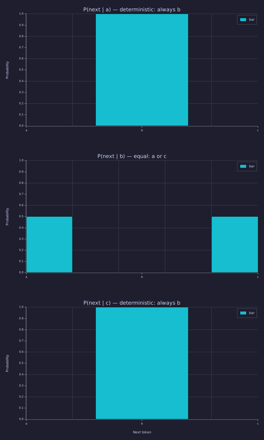
Each panel is one row of \(\mathbf{P}\) — the distribution the model samples from when it sits at that token. The two single-bar panels have zero entropy; the middle one carries the model's only bit of uncertainty.
Engineering Lenses
No signals reading adds to this lesson: the count matrix is a two-dimensional histogram of transitions, and that is all a signals view would say. The systems and information readings are both exact.
Systems
Exact. Let \(\boldsymbol{\pi}_t \in \mathbb{R}^{1 \times |\mathcal{V}|}\) be the distribution of the token at time \(t\). The bigram model's update law is
\[\boldsymbol{\pi}_{t+1} = \boldsymbol{\pi}_t \mathbf{P},\]
a discrete-time linear time-invariant system whose state lives on the probability simplex. Row-stochasticity fixes its spectrum: \(\mathbf{P}\mathbf{1} = \mathbf{1}\), so \(\lambda = 1\) is an eigenvalue, and no eigenvalue can exceed 1 in modulus (Gershgorin: every row sums to 1). The spectral radius is exactly 1 — marginal stability by construction — and the left eigenvector for \(\lambda = 1\), \(\boldsymbol{\pi}\mathbf{P} = \boldsymbol{\pi}\), is the stationary distribution, the system's fixed point. The remaining eigenvalues decide whether \(\boldsymbol{\pi}_t\) converges to it. eig(P') returns the left eigenvectors of \(\mathbf{P}\):
[V, D] = eig(P');                       % columns of V: left eigenvectors of P
lam = real(diag(D));                    % eig returns vectors — no transpose needed
k1 = argmax(lam);                       % the lambda = 1 mode
pi_st = real(V(:, k1));
pi_st = pi_st / sum(pi_st);             % normalise to a distribution
print("eigenvalues of P      :", lam);
print("stationary pi         :", pi_st);
print("pi * P                :", pi_st * P);
print("empirical unigram     :", [sum(seq == 1), sum(seq == 2), sum(seq == 3)] / n_tokens);

lam_s = eig(P_smooth');
[Vs, Ds] = eig(P_smooth');
ks = argmax(real(diag(Ds)));
pi_sm = real(Vs(:, ks));
pi_sm = pi_sm / sum(pi_sm);
abs_s = reshape(sort(abs(lam_s), "descend"), 1, vocab_size);
print("|eigenvalues| P_smooth:", abs_s);
print("stationary pi (smooth):", pi_sm);
print("mixing |lambda_2|^8 =", abs_s(2) ^ 8);eigenvalues of P : [1×3] 1.000000 0.000000 -1.000000
stationary pi : [1×3] 0.250000 0.500000 0.250000
pi * P : [1×3] 0.250000 0.500000 0.250000
empirical unigram : [1×3] 0.333333 0.444444 0.222222
|eigenvalues| P_smooth: [1×3] 1.000000 0.457143 0.000000
stationary pi (smooth): [1×3] 0.294118 0.411765 0.294118
mixing |lambda_2|^8 = 0.0019072846188029414The spectrum is \(\{1, 0, -1\}\). The eigenvalue at \(-1\) is a pole on the unit circle: a marginally stable period-2 mode. Starting from \(\mathbf{e}_a\), one step gives \(\mathbf{e}_b\), the next \([\tfrac12, 0, \tfrac12]\), then \(\mathbf{e}_b\) again — the distribution itself alternates forever and never settles to \(\boldsymbol{\pi} = [\tfrac14, \tfrac12, \tfrac14]\). That is why b occupies every even position of the sample, and why the empirical unigram \([3, 4, 2]/9\) of the corpus is not \(\boldsymbol{\pi}\): a periodic chain has a stationary distribution but no limiting one; only its time average converges. Add-one smoothing puts an edge on every pair of states, the pole at \(-1\) moves inside the circle to \(|\lambda_2| = 0.457\), and the chain becomes ergodic: it mixes at rate \(|\lambda_2|^t\) (time constant \(-1/\ln|\lambda_2| \approx 1.28\) steps), so after eight steps the transient has decayed to \(0.0019\) of its size and \(\boldsymbol{\pi}_t\) sits on \(\boldsymbol{\pi}^{\text{smooth}} = [5, 7, 5]/17\).
% pi_t = e_a P^t for t = 0..8.  (P^k is element-wise in rustlab — iterate instead.)
n_steps = 8;
traj   = zeros(n_steps + 1, vocab_size);
traj_s = zeros(n_steps + 1, vocab_size);
row = [1, 0, 0];  row_s = [1, 0, 0];
for t = 0:n_steps
  traj(t + 1, :)   = row;
  traj_s(t + 1, :) = row_s;
  row   = row * P;
  row_s = row_s * P_smooth;
end
steps = 0:n_steps;

figure();
subplot(1, 2, 1)
hold("on")
plot(steps, traj(:, 1)', "color", "blue",  "label", "P(a)")
plot(steps, traj(:, 2)', "color", "red",   "label", "P(b)")
plot(steps, traj(:, 3)', "color", "green", "label", "P(c)")
yline(pi_st(2), "gray", "pi(b) = 0.5")
legend("P(a)", "P(b)", "P(c)")
title("pi_t under P: pole at -1, period 2")
xlabel("t"); ylabel("probability")
hold("off")
subplot(1, 2, 2)
hold("on")
plot(steps, traj_s(:, 1)', "color", "blue",  "label", "P(a)")
plot(steps, traj_s(:, 2)', "color", "red",   "label", "P(b)")
plot(steps, traj_s(:, 3)', "color", "green", "label", "P(c)")
yline(pi_sm(2), "gray", "pi(b) = 7/17")
legend("P(a)", "P(b)", "P(c)")
title("pi_t under P_smooth: |lambda_2| = 0.457")
xlabel("t"); ylabel("probability")
hold("off")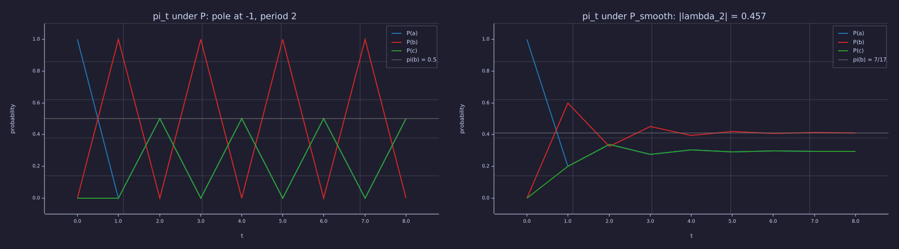
Left: \(P(b)\) flips between 0 and 1 on every step and never approaches the dashed stationary value — the \(-1\) pole. Right: the same start under \(\mathbf{P}^{\text{smooth}}\) decays onto the dashed line in about three steps, alternating in sign as a negative real pole should.
Information
Exact. The entropy rate of the stationary chain is the row entropies averaged under \(\boldsymbol{\pi}\), and the maximum-likelihood \(\mathbf{P}\) makes the training cross-entropy equal to it — MLE is minimum cross-entropy. The two agree to the last digit here because the corpus is a closed walk (it starts and ends on a), so the empirical frequency of the current token is exactly the stationary \(\boldsymbol{\pi}\):
H_rate  = sum(pi_st .* H_rows);
ce_bits = mean_ce / log(2);
H_uni   = entropy_bits([sum(seq == 1), sum(seq == 2), sum(seq == 3)] / n_tokens);
print("entropy rate sum_i pi_i H_i =", H_rate, "bits");
print("training CE (bits), raw P  =", ce_bits, "   P_smooth =", mean_ce_smooth / log(2));
print("floors: log2|V| =", log2(vocab_size), "  H(unigram) =", H_uni, "  H(next|cur) =", H_rate);

figure();
bar({"log2|V| blind", "H(X) unigram", "H(next|cur) bigram"}, [log2(vocab_size), H_uni, H_rate])
title("Staircase of floors for 'abcbabcba' (bits per token)")
ylabel("bits")
ylim([0, 1.8])entropy rate sum_i pi_i H_i = 0.5000000000000001 bits
training CE (bits), raw P = 0.5 P_smooth = 0.979679007751327
floors: log2|V| = 1.584962500721156 H(unigram) = 1.5304930567574824 H(next|cur) = 0.5000000000000001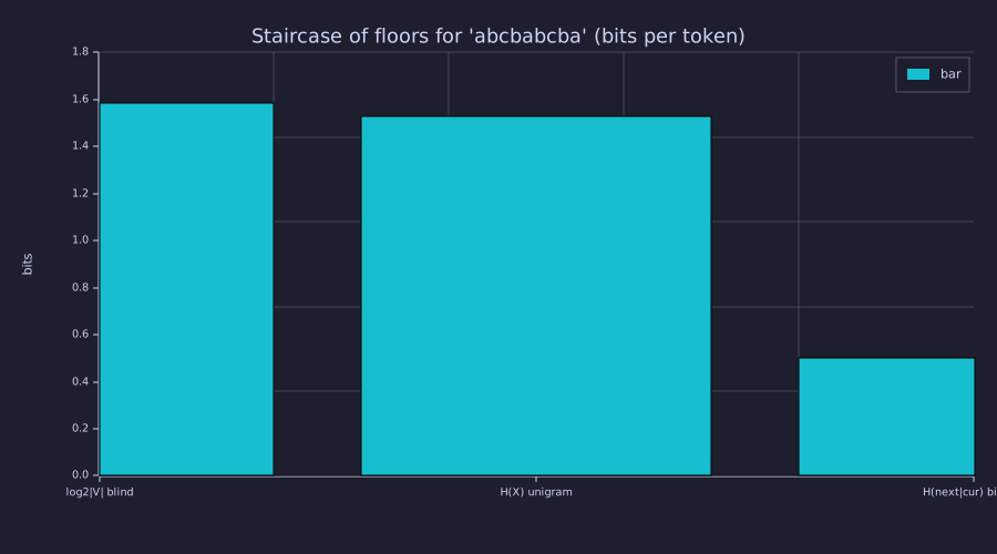
Each step down is information a stronger model class recovers: \(\log_2 3 = 1.585\) bits for a blind guess, \(1.530\) bits knowing only letter frequencies, \(0.500\) bits knowing the previous letter. 23-putting-it-all-together adds the trained transformer's cross-entropy as the next step.
The staircase is the chain rule of entropy made visible. Because conditioning cannot increase entropy, \(H(X_{t+1} \mid X_t) \ge H(X_{t+1} \mid X_1, \ldots, X_t)\): the bigram's \(0.5\) bits is a ceiling for any longer-context model of this corpus and a floor for any model that sees only the current token — Shannon's source-coding theorem says no such code can beat it. Every later lesson — attention, the transformer, the capstone — is a method to recover the entropy that the Markov assumption leaves on the table. Perplexity is the same number in a different base: \(2^{0.5} = e^{0.3466} = 1.414\) effective choices per step. And the equivalence with compression is literal: feed these conditional distributions to an arithmetic coder and the corpus compresses to \(0.5\) bits per token plus a constant; the smoothed model would spend \(0.98\).
Key Takeaways
- The bigram model encodes corpus statistics in a single row-stochastic matrix — reading a row tells you exactly what the model "thinks" will follow a given token; dividing counts by row sums is the maximum-likelihood estimate.
- Inverse-transform sampling from a row of \(\mathbf{P}\) is the primitive every sampling strategy in Lesson 21 (temperature, top-K, nucleus) is built on.
- The training cross-entropy of the MLE equals the conditional entropy \(\sum_i \pi_i H(\mathbf{P}_{i,:})\) — here \(0.5\) bits, perplexity \(1.414\); smoothing trades training fit (\(0.98\) bits) for finite loss on unseen bigrams.
- \(\boldsymbol{\pi}_{t+1} = \boldsymbol{\pi}_t \mathbf{P}\) is a linear system with spectral radius 1: the \(\lambda = 1\) left eigenvector is the stationary distribution, and any other eigenvalue on the unit circle (here \(-1\)) is a mode that never dies out. Smoothing pulls it inside and the chain mixes.
- Its weakness: context is limited to one token. The bigram's entropy rate is a floor for Markov-1 models and a ceiling for everything that follows.
Standalone Scripts
| Script | What it computes |
|---|---|
bigram_counts.rlab | the 3×3 bigram count, one-line row-normalised, and smoothed probability matrices for "abcbabcba"; row entropies and \(H(X_{t+1}\mid X_t)\); heatmaps |
bigram_sampling.rlab | inverse-transform sampling trace, a 12-token generated sequence decoded to text, training CE under \(\mathbf{P}\) and \(\mathbf{P}^{\text{smooth}}\) |
bigram_stationary.rlab | eig(P') → stationary distribution and the \(\{1, 0, -1\}\) spectrum; \(\boldsymbol{\pi}_t\) under \(\mathbf{P}\) vs \(\mathbf{P}^{\text{smooth}}\); entropy rate and the staircase of floors |
Run all with make lesson-05 (or rustlab run lessons/05-bigram-language-model/<name>.rlab).
Expected Numerical Outputs Summary
| Variable | Expected Value |
|---|---|
n_tokens, n_bigrams | 9, 8 |
sum(sum(C)) | 8 (= n_bigrams) |
P(1, 2), P(2, 1), P(2, 3) | 1.0, 0.5, 0.5 |
min_smooth | ≈ 0.143 (= 1/7, the b → b cell) |
H_rows | [0, 1, 0] bits |
pi_emp | [0.25, 0.5, 0.25] |
H_cond | 0.5 bits |
gen_text (seed 7) | ababcbcbabcb |
mean_ce, ppl | 0.3466 nats (= 0.5 bits), 1.414 |
mean_ce_smooth | 0.679 nats (= 0.980 bits), ppl 1.972 |
eig(P') | {1, 0, -1} |
pi_st | [0.25, 0.5, 0.25] |
abs(eig(P_smooth')) (sorted) | {1, 0.457, 0}; 0.457^8 ≈ 0.0019 |
pi_sm | [0.294, 0.412, 0.294] (= [5, 7, 5]/17) |
H_rate | 0.5 bits (= ce_bits) |
log2(3), H_uni | 1.585, 1.530 bits |
Exercises
- Entropy of rows. The notebook prints \(H(a), H(b), H(c)\) for
"abcbabcba". Which token is most predictable? Which is least? Repeat for the corpus"aabbcc"— the one-line normalisation works unchanged for any \(|\mathcal{V}|\). - Laplace smoothing effect. For
"abcbabcba"with \(|\mathcal{V}| = 3\), compute the Laplace-smoothed probability for the bigram (a → a), which never appeared. What is \(P^{\text{smooth}}_{11}\), and what happens to the training cross-entropy under add-\(k\) smoothing as \(k \to \infty\)? - Longer corpus. Extend the corpus to
"abcbabcbabc"and recompute the bigram matrix. Do the probabilities change significantly? What happens as the corpus grows? - Perplexity interpretation. What does a perplexity of 1 mean? What about perplexity of \(|\mathcal{V}|\)? Check that \(2^{\mathcal{L}_{\text{bits}}}\) and \(e^{\mathcal{L}_{\text{nats}}}\) agree on this corpus.
- Beyond bigrams. A trigram model conditions on the last two tokens: \(P(x_{t+1} \mid x_{t-1}, x_t)\). How many parameters does a trigram model have for vocabulary size \(|\mathcal{V}|\)? How does this scale compared to the bigram model?
- Spectral gap. Replace add-one by add-\(k\) for \(k \in \{0.01, 0.1, 1, 10\}\) and print \(|\lambda_2|\) of \(\mathbf{P}^{\text{smooth}}\) each time. Which way does the pole move as \(k \to 0\), and what does that say about how quickly a lightly smoothed chain forgets its starting token?
Solution to 6 (sketch)
As \(k \to 0\) the smoothed matrix approaches \(\mathbf{P}\) and \(|\lambda_2| \to 1\): the pole returns to the unit circle and the mixing time \(-1/\ln|\lambda_2|\) diverges. As \(k \to \infty\) every row tends to the uniform distribution, \(\mathbf{P}^{\text{smooth}} \to \tfrac13 \mathbf{1}\mathbf{1}^\top\), whose non-unit eigenvalues are all zero — the chain forgets its start in a single step.
What's next
06-linear-layers-and-gradient-descent replaces the count table with a learned linear layer \(\mathbf{y} = \mathbf{x}\mathbf{W} + \mathbf{b}\) and shows how gradient descent drives the parameters toward the same optimum the count-based estimator finds analytically. The transition from "look up" to "learn" is the conceptual jump from a classical n-gram model to a neural one — every subsequent lesson uses gradient descent.