Lesson 01: Tokens & Text Encoding
A language model never sees letters — it sees integers. This lesson builds the bridge from raw text to the numerical representations every later lesson depends on: a vocabulary, an executed encode/decode round trip, one-hot vectors, and the first two information-theoretic floors that every model in this course will be measured against. One corpus — "to be or not to be" — runs through the whole lesson.
Learning Objectives
- Explain what a token is and why text must be converted to numbers before a model can process it.
- Build a character-level vocabulary, then encode a string to integer ids and decode it back, in executed code.
- Construct a one-hot vector for a given token, interpret it as a standard basis vector, and stack a sequence into the matrix \(\mathbf{X} \in \{0,1\}^{T \times |\mathcal{V}|}\).
- Read a character PMF bar chart and a one-hot matrix heatmap and explain what each cell means.
- Compute the first two floors on the entropy staircase — \(\log_2 |\mathcal{V}|\) and the unigram entropy \(H(f)\) — and say what later lessons must do to go lower.
Background
Vectors (a list of numbers) and matrices (a 2-D grid of numbers). The concept of a function as a deterministic input-to-output mapping. Base-2 logarithms. No neural network, probability, or deep learning knowledge is required yet — those arrive in later lessons.
What is a Token?
Theory
A token is the basic unit of text a language model operates on. At the character level every character becomes one token. The pipeline this lesson builds — and the one box it borrows from 04-embeddings-and-similarity — is:
Step 1 — Collect the vocabulary. Given a corpus, collect every unique character and sort them. This ordered set is the vocabulary \(\mathcal{V}\), with size \(|\mathcal{V}|\) (written \(V\) on diagram edges).
Step 2 — Assign integer indices. Create a deterministic mapping and its inverse
\[\text{encode} : \mathcal{V} \to \{1, 2, \ldots, |\mathcal{V}|\}, \qquad \text{decode} = \text{encode}^{-1}.\]
For the corpus "to be or not to be" the sorted vocabulary is:
| Character | Index |
|---|---|
␣ (space) | 1 |
b | 2 |
e | 3 |
n | 4 |
o | 5 |
r | 6 |
t | 7 |
Encoding is lossless: \(T\) characters become \(T\) integers \(x(1), \ldots, x(T)\) in \(1..|\mathcal{V}|\), and decoding recovers the text exactly. The index \(t = 1, \ldots, T\) is discrete time — the axis every later lesson calls the sequence.
Example — Encode and decode round trip
Rustlab strings index by character (s(t)), so the encoder is a search for each character's position in the vocabulary; the decoder is a string concatenation of chars(ids(t)):
corpus = "to be or not to be";
chars  = {" ", "b", "e", "n", "o", "r", "t"};        % sorted vocabulary
vocab_size = length(chars);
T = length(corpus);

% encode: ids(t) = position of corpus(t) in the vocabulary
ids = zeros(T);
for t = 1:T
  j = 1;
  while j < vocab_size && corpus(t) != chars(j)
    j = j + 1;
  end
  ids(t) = j;
end

% decode: concatenate the vocabulary entry for each id
decoded = "";
id_str  = "";
for t = 1:T
  decoded = decoded + chars(ids(t));
  id_str  = id_str + sprintf("%d ", ids(t));
end

print("T =", T, " |V| =", vocab_size);
print("ids:      ", id_str);
print("decoded:  '" + decoded + "'");
print("round trip exact:", decoded == corpus);T = 18 |V| = 7
ids: 7 5 1 2 3 1 5 6 1 4 5 7 1 7 5 1 2 3
decoded: 'to be or not to be'
round trip exact: trueThe corpus has \(T = 18\) characters over a vocabulary of \(|\mathcal{V}| = 7\); t is id 7 and o is id 5, so the text opens 7 5 1 .... Every later lesson consumes a sequence like ids — 05-bigram-language-model counts transitions in a sequence like it, 18-training-loop trains on one.
Character Frequencies
Theory
Before building a model it helps to understand the frequency distribution of tokens. If \(c_i\) is the count of character \(i\) in the corpus, the relative frequency is
\[f_i = \frac{c_i}{\sum_{j=1}^{|\mathcal{V}|} c_j}.\]
This is a discrete probability distribution — a PMF — over the vocabulary: every \(f_i \in [0, 1]\) and \(\sum_i f_i = 1\). It is the first-order marginal of the corpus: the probability of a character with no knowledge of its neighbours.
Example — Counting from the id sequence and the PMF bar chart
The counts come from the encoded ids, not from a hand-typed table:
counts = zeros(vocab_size);
for t = 1:T
  counts(ids(t)) = counts(ids(t)) + 1;
end
total = sum(counts);
freqs = counts / total;
print("Character counts (␣, b, e, n, o, r, t):", counts);
print("Relative frequencies:", freqs);
print("Sum of frequencies (should be 1.0):", sum(freqs));

labels = {"␣", "b", "e", "n", "o", "r", "t"};
figure();
bar(labels, freqs, "Character PMF f_i: 'to be or not to be'")
ylim([0, 0.3])Character counts (␣, b, e, n, o, r, t): [1×7] 5.000000 2.000000 2.000000 1.000000 4.000000 1.000000 3.000000
Relative frequencies: [1×7] 0.277778 0.111111 0.111111 0.055556 0.222222 0.055556 0.166667
Sum of frequencies (should be 1.0): 1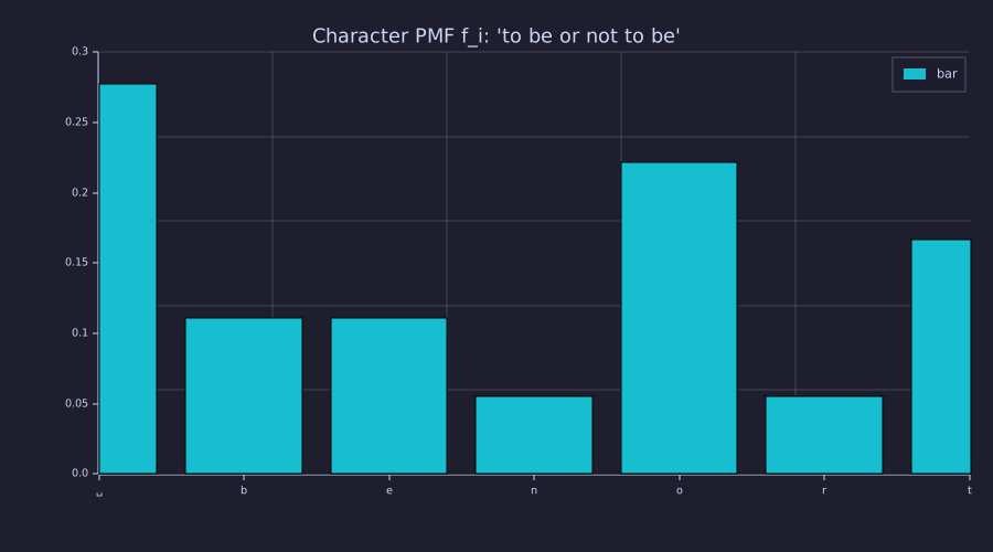
The first bar is the space character ␣ — the most frequent symbol at 0.278 \(= 5/18\). The bar heights sum to 1.0; this PMF is the "unigram source" whose entropy is computed under Engineering Lenses below.
One-Hot Encoding
Theory
An integer index like \(4\) carries no useful geometric meaning — a model might infer that character 4 is "greater than" character 3, which is meaningless. Instead, each token is represented as a one-hot vector: a vector of length \(|\mathcal{V}|\) that is 0 everywhere except at position \(i\):
\[(\mathbf{e}_i)_j = \begin{cases} 1 & \text{if } j = i \\ 0 & \text{otherwise.} \end{cases}\]
\(\mathbf{e}_i\) is row \(i\) of the identity matrix \(\mathbf{I}_{|\mathcal{V}|}\) — the \(i\)-th standard basis vector. All one-hot vectors are therefore mutually orthogonal:
\[\mathbf{e}_i \cdot \mathbf{e}_j = \delta_{ij}.\]
No two tokens share any geometric similarity — a clean slate before the model learns its own representations (04-embeddings-and-similarity).
To encode a sequence of \(T\) tokens, stack their one-hot vectors as rows of a matrix \(\mathbf{X} \in \{0, 1\}^{T \times |\mathcal{V}|}\) — tokens are rows (time), vocabulary slots are columns:
\[\mathbf{X} = \begin{bmatrix} \mathbf{e}_{x(1)} \\ \mathbf{e}_{x(2)} \\ \vdots \\ \mathbf{e}_{x(T)} \end{bmatrix}.\]
Example — Stacking one-hots into a matrix X
Because \(\mathbf{e}_i\) is row \(i\) of the identity, the whole matrix is one row gather; the same block checks orthogonality and the fact Lesson 04 builds on — \(\mathbf{X}\) times a matrix selects rows of it:
I = eye(vocab_size);
X = I(ids, :);                          % row t of X is e_{ids(t)}

print("X is", size(X, 1), "x", size(X, 2), " (T tokens x |V| slots)");
print("First five rows of X  ('to be'):");
print(X(1:5, :));
print("Fraction of non-zero entries:", sum(sum(X)) / (T * vocab_size), " = 1/|V| =", 1 / vocab_size);

e_t = I(7, :);  e_o = I(5, :);
dot_t_o = sum(e_t .* e_o);
dot_t_t = sum(e_t .* e_t);
lookup_diff = max(max(abs(X * eye(vocab_size) - X)));
print("Dot product t . o:", dot_t_o, "   t . t:", dot_t_t);
print("max|X * eye(|V|) - X| :", lookup_diff);X is 18 x 7 (T tokens x |V| slots)
First five rows of X ('to be'):
Matrix(5x7)
[0.000000, 0.000000, 0.000000, 0.000000, 0.000000, 0.000000, 1.000000]
[0.000000, 0.000000, 0.000000, 0.000000, 1.000000, 0.000000, 0.000000]
[1.000000, 0.000000, 0.000000, 0.000000, 0.000000, 0.000000, 0.000000]
[0.000000, 1.000000, 0.000000, 0.000000, 0.000000, 0.000000, 0.000000]
[0.000000, 0.000000, 1.000000, 0.000000, 0.000000, 0.000000, 0.000000]
Fraction of non-zero entries: 0.14285714285714285 = 1/|V| = 0.14285714285714285
Dot product t . o: 0 t . t: 1
max|X * eye(|V|) - X| : 0The matrix is 18 \(\times\) \(7\) — one row per token, one column per vocabulary slot. Each row has exactly one non-zero entry, so only \(1/|\mathcal{V}| = 0.143\) of the matrix is non-zero; at a realistic \(|\mathcal{V}| = 50{,}000\) that density is \(0.002\,\%\), which is why real implementations never materialise \(\mathbf{X}\). Orthogonality is confirmed — \(\mathbf{e}_t \cdot \mathbf{e}_o = 0\), \(\mathbf{e}_t \cdot \mathbf{e}_t = 1\), exactly \(\delta_{ij}\) — and \(\mathbf{X}\,\mathbf{I} = \mathbf{X}\) to the last bit: row \(t\) of \(\mathbf{X}\mathbf{M}\) is row \(x(t)\) of \(\mathbf{M}\) for any matrix \(\mathbf{M}\) with \(|\mathcal{V}|\) rows. Replace \(\mathbf{I}\) by a \(|\mathcal{V}| \times d\) matrix \(\mathbf{E}\) and you have the embedding lookup of 04-embeddings-and-similarity.
Example — One-hot matrix heatmap
seq_labels = labels(ids);                % the character at each position

figure();
heatmap(labels, seq_labels, X, "One-Hot Matrix X: 'to be or not to be' (18 tokens x 7 slots)", "viridis")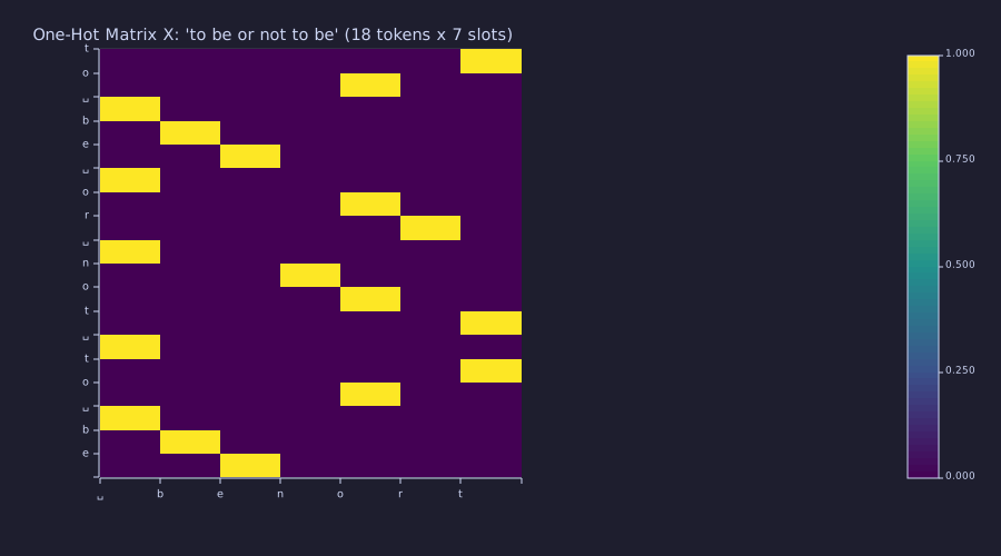
Read each row left to right: the single bright cell sits under the column for that row's character, so the picture is the encoding. The five ␣ rows all light the first column — identical tokens have identical rows.
Engineering Lenses
No systems reading adds to this lesson: tokenisation has no state and no update law. The first state variable of the course is the Markov chain of 05-bigram-language-model.
Signals
Exact. The signal is the symbol stream \(x(t)\), \(t = 1, \dots, T\), on the discrete-time axis; its values live on a second discrete axis, the alphabet index \(i = 1, \dots, |\mathcal{V}|\). On that alphabet axis a one-hot vector is the unit impulse \(\mathbf{e}_i[n] = \delta[n - i]\) — the same object as the standard basis vector — and the PMF \(f\) is a finite sequence over the same axis. \(\mathbf{X}\) is then \(T\) impulses, one per row.
figure();
subplot(1, 2, 1)
stem(1:vocab_size, freqs)
title("PMF f[i] over the alphabet index i (1 = ␣)")
ylim([0, 0.3])
subplot(1, 2, 2)
stem(1:vocab_size, X(1, :))
title("one-hot of x(1) = 't':  delta[n - 7]")
ylim([0, 1.1])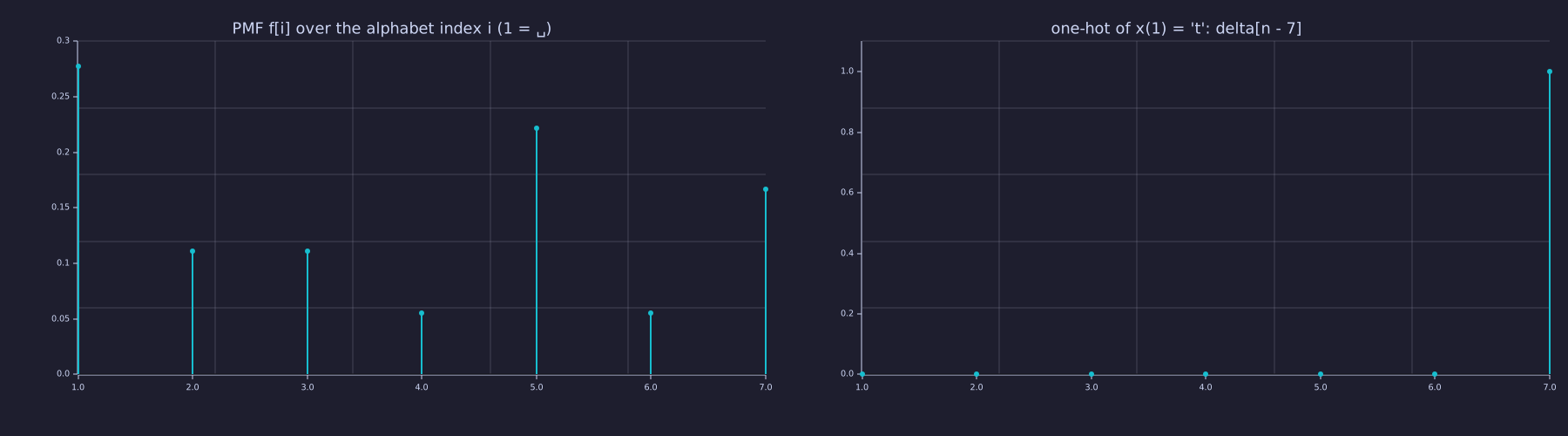
Same axis, two sequences: the left stem plot is a distribution over the alphabet, the right one is a single impulse at \(n = 7\). Every row of \(\mathbf{X}\) is an impulse like the right panel; Lesson 04 replaces the impulse by a dense \(d\)-vector.
Information
Exact. The corpus is a realisation of a discrete source \(X_t\) over the alphabet \(\mathcal{V}\), and \(f\) is its empirical first-order marginal. Shannon's source-coding theorem says the minimum average number of bits to losslessly encode symbols drawn independently from \(f\) is the entropy
\[H(f) = -\sum_{i=1}^{|\mathcal{V}|} f_i \log_2 f_i \quad [\text{bits/symbol}].\]
Every \(f_i > 0\) here, so the sum needs no special case (the \(0 \log 0 = 0\) convention is stated in 02-probability-and-softmax, which formalises entropy; later lessons call lib/info.rlab):
H_f   = -sum(freqs .* log2(freqs));      % unigram (memoryless) entropy, bits/symbol
H_max = log2(vocab_size);                % uniform-alphabet bound

print("log2|V|      =", H_max, "bits/symbol");
print("H(f) unigram =", H_f, "bits/symbol");
print("gap =", H_max - H_f, "bits/symbol");log2|V| = 2.807354922057604 bits/symbol
H(f) unigram = 2.594117891631186 bits/symbol
gap = 0.21323703042641817 bits/symbolTwo reference points, both in bits per symbol: if every character were equally likely each token would carry \(\log_2 7 = 2.807\) bits; with the actual frequencies the bound is \(H(f) = 2.594\) bits — \(0.213\) bits less per token. A variable-length code (Huffman, arithmetic) can approach \(H(f)\); a fixed-width binary code cannot split a bit and rounds up to \(\lceil \log_2 7 \rceil = 3\).
Exact. \(H(f)\) is the memoryless floor: it assumes each character is drawn independently of its neighbours. Conditioning on the previous character can only lower it, \(H(X_{t+1} \mid X_t) \le H(X_{t+1})\), and conditioning on the whole past lowers it further. This course is a staircase of such floors, each model class beating the last. The third step — the bigram conditional entropy — is derived in 05-bigram-language-model; it is computed here ahead of its derivation, from the transition counts of this corpus, so the staircase can be drawn:
C = zeros(vocab_size, vocab_size);       % C(i, j): count of (x(t) = i, x(t+1) = j)
for t = 1:T - 1
  C(ids(t), ids(t + 1)) = C(ids(t), ids(t + 1)) + 1;
end
H_cond = 0;                              % -sum_ij p(i,j) log2 p(j|i)
for i = 1:vocab_size
  for j = 1:vocab_size
    if C(i, j) > 0
      H_cond = H_cond - (C(i, j) / (T - 1)) * log2(C(i, j) / sum(C(i, :)));
    end
  end
end
print("H(X_{t+1} | X_t) bigram preview =", H_cond, "bits/symbol");

figure();
bar({"uniform log2|V|", "unigram H(f)  (L01)", "bigram"}, [H_max, H_f, H_cond], "The staircase of floors (bits/token)")
ylim([0, 3])H(X_{t+1} | X_t) bigram preview = 1.0802663515647224 bits/symbol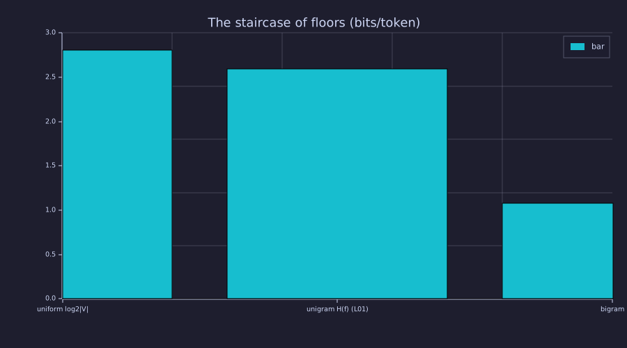
Left to right: uniform alphabet \(2.807\) → unigram \(2.594\) → bigram \(H(X_{t+1} \mid X_t) = 1.080\) bits per token (the third bar is Lesson 05's floor). The fourth step, the trained transformer of 23-putting-it-all-together, is measured on a different corpus and so is not drawn here; its cross-entropy in bits is the same kind of number and sits below the bigram floor of its corpus.
Exact. One-hot encoding is a one-of-N code: it spends \(|\mathcal{V}|\) binary digits to carry at most \(\log_2 |\mathcal{V}|\) bits — like writing the number 5 as 0000100 instead of 101 — with redundancy \(1 - \log_2|\mathcal{V}| / |\mathcal{V}|\). And tokenisation changes the symbol rate, not the message: the same 18-character message is 6 word-level symbols, and what a tokeniser trades is symbols per message against bits per symbol:
redundancy = 1 - H_max / vocab_size;
print("one-hot redundancy 1 - log2|V|/|V| =", redundancy);

% word level: to, be, or, not, to, be  ->  vocabulary {be, not, or, to}
f_words = [2, 1, 1, 2] / 6;
H_words = -sum(f_words .* log2(f_words));
bits_chars = T * H_f;
bits_words = 6 * H_words;
print("chars: 18 symbols x", H_f, "bits =", bits_chars, "bits/message");
print("words: 6 symbols x", H_words, "bits =", bits_words, "bits/message");one-hot redundancy 1 - log2|V|/|V| = 0.5989492968489136
chars: 18 symbols x 2.594117891631186 bits = 46.69412204936135 bits/message
words: 6 symbols x 1.9182958340544896 bits = 11.509775004326936 bits/messageThe redundancy is \(0.599\) at \(|\mathcal{V}| = 7\) and \(0.9997\) at \(50{,}000\); we accept it because one-hot vectors plug directly into matrix algebra, and the embedding of Lesson 04 is the dense code that trades it away. The two memoryless products disagree — \(46.7\) versus \(11.5\) bits for the same message — and the gap is mostly the information the character-level memoryless source cannot see: that t is followed by o, that b is followed by e (the rest is bookkeeping — the word-level count drops the spaces and ignores dependence between words). A model that captured every dependency would give the same bits per message under either tokenisation, because the information in a message does not depend on how it is chopped up. Bigger symbols push bits into the symbol table, smaller symbols push them into the sequence model — the trade 19-byte-pair-encoding makes explicit; 03-cross-entropy-loss measures the bits per token a model wastes against the floor, and 20-perplexity-and-evaluation reads \(2^{H}\) as an effective alphabet size.
Key Takeaways
- Tokenisation converts symbols to integers to matrices — the bridge from text to linear algebra — and it is lossless:
decode(encode(s)) == s. - A character-level vocabulary is tiny (~100 in English) but forces the model to learn spelling from scratch. Larger vocabularies reduce sequence length but increase memory.
- One-hot vectors are the standard basis of \(\mathbb{R}^{|\mathcal{V}|}\); \(\mathbf{X}\mathbf{M}\) selects rows of \(\mathbf{M}\). One-hot encoding does not imply characters are independent — it is only the starting point. The embedding layer (04-embeddings-and-similarity) projects these orthogonal vectors into a dense space where learned relationships emerge.
- The staircase of floors starts here: \(\log_2|\mathcal{V}| = 2.807 \to H(f) = 2.594 \to H(X_{t+1}\mid X_t) = 1.080\) bits per token on this corpus. Every later model is judged by how far down it gets.
Standalone Scripts
| Script | What it computes |
|---|---|
encode_decode.rlab | the vocabulary, the encode/decode round trip, and counts/frequencies from the id sequence |
char_frequencies.rlab | character counts and relative frequencies for "to be or not to be"; labelled PMF bar chart |
one_hot_encoding.rlab | the 18×7 one-hot matrix from the ids; density, orthogonality, the X * eye lookup; heatmap |
entropy_floors.rlab | \(\log_2\lvert\mathcal{V}\rvert\), \(H(f)\), the bigram preview, one-hot redundancy, the symbol-rate comparison; staircase bar chart |
Run all with make lesson-01 from the repo root (or rustlab run lessons/01-tokens-and-encoding/<name>.rlab for one). Each writes SVGs next to the script (gitignored).
Expected Numerical Outputs Summary
| Variable | Expected Value |
|---|---|
T, vocab_size | 18, 7 |
ids (first five) | 7 5 1 2 3 ("to be"); decoded == corpus is true |
freqs (max — space), sum(freqs) | ≈ 0.278 (= 5/18), 1.0 |
size(X), non-zero fraction | [18, 7], 0.143 (= 1/7) |
dot_t_o, dot_t_t, lookup_diff | 0, 1, 0 |
H_max, H_f, H_cond | 2.807, 2.594, 1.080 bits/symbol |
redundancy | 0.599 |
bits_chars, bits_words | 46.7, 11.5 bits/message |
Exercises
- Vocabulary extension. Modify
encode_decode.rlabto use the corpus"the cat sat on the mat". What is the new vocabulary size? Which character has the highest frequency, and what is \(H(f)\)? - Decode a sequence. Using this lesson's vocabulary, decode
[4, 5, 7, 1, 7, 5]by hand, then check with thedecodedloop. - One-hot orthogonality. Compute the dot product between row 1 (
t) and row 4 (b) of \(\mathbf{X}\) by hand, and the dot product between rows 1 and 14 (botht). Confirm both against \(\delta_{ij}\). - Vocabulary size trade-off. The one-hot matrix for \(T\) tokens over \(N\) symbols has \(T \times N\) entries, of which \(T\) are non-zero. Write the density and the one-of-N code redundancy as formulas in \(N\); evaluate both at \(N = 7\), \(256\), \(50{,}000\).
- Beyond characters. Tokenise
"to be or not to be"at the word level. What are \(T\) and \(|\mathcal{V}|\) now, what is the shape of \(\mathbf{X}\), and does \(T \cdot H(f)\) go up or down? Reconcile your answer with the symbol-rate block above.
What's next
02-probability-and-softmax turns scores into a probability distribution over the vocabulary with the softmax function — derived as the maximum-entropy distribution, not merely constructed — and introduces the temperature \(\tau\) that controls how sharp or diffuse the distribution is. The entropy computed here reappears there as a function of \(\tau\).