Lesson 09: Multi-Head Attention
A single attention head (08-scaled-dot-product-attention) produces one row-stochastic mixing matrix \(\mathbf{A}\). Language has many kinds of relationships — syntactic, positional, coreferential — and one head can express only one of them per position. Multi-head attention runs \(H\) heads in parallel, concatenates their outputs, and projects them back to model width. In signal-processing terms it is a filter bank: \(H\) causal time-varying filters, each applied to its own low-rank slice of the signal, summed through a synthesis matrix \(\mathbf{W}_O\).
Learning Objectives
- Explain why a single attention head is limited (one softmax gives one convex combination per position, and its score matrix has rank at most \(d_k\)) and what multi-head attention (MHA) buys at the same cost.
- Compute \(H\) parallel attention heads \(\mathbf{A}_1, \dots, \mathbf{A}_H\), each with its own \(\mathbf{W}_Q^h, \mathbf{W}_K^h, \mathbf{W}_V^h\), on the same input \(\mathbf{X}\).
- Write the concatenation of per-head outputs as a horizontal stack along the feature axis, apply the output projection \(\mathbf{W}_O\), and verify the filter-bank identity \(\mathrm{Concat}\cdot\mathbf{W}_O = \sum_h \mathbf{A}_h \mathbf{X} \mathbf{W}_V^h \mathbf{W}_O^{(h)}\) numerically.
- Derive the total parameter count of an MHA block as \(4 d_{\text{model}}^2\) when \(d_k = d_v = d_{\text{model}}/H\).
- Read a grid of head-attention heatmaps as four causal filters (first-sample hold, unit delay, identity, growing box) and measure each head's selectivity in bits.
Background
Scaled dot-product attention, the causal mask, and the \(\mathbf{Q}, \mathbf{K}, \mathbf{V}\) formulation from 08-scaled-dot-product-attention. Linear layers and matrix multiplication from 06-linear-layers-and-gradient-descent. Block-wise horizontal concatenation of matrices. Row entropy of a stochastic matrix in bits (lib/info.rlab, applied to attention in Lesson 08).
Why More Than One Head
Theory
A single attention head can compute one way of relating tokens — for example, "each token attends to the previous one". But language has many relationships: syntactic (subject–verb agreement), coreference (it → mat), long-range dependencies (quotes), positional (first token, last token). Two structural limits make one head insufficient:
- One softmax, one convex combination. Row \(t\) of \(\mathbf{A}\) is a single probability vector over the past, so the output at \(t\) is one weighted average of the values. A head cannot fetch "the previous token" and "the first token" as separate quantities; it can only blend them.
- Rank at most \(d_k\). The score matrix \(\mathbf{Q}_h\mathbf{K}_h^\top\) is a product of two \(T \times d_k\) factors, so its rank is at most \(d_k\): a narrow head chooses its pattern from a \(d_k\)-dimensional family (verified in the Signals lens below).
Multi-head attention runs \(H\) independent attention computations in parallel, each with its own projection matrices, and combines the results. \(H\) heads of width \(d_k = d_{\text{model}}/H\) cost the same multiply–adds as one head of width \(d_{\text{model}}\) (the score FLOPs are \(2T^2 d_{\text{model}}\) either way) but perform \(H\) simultaneous retrievals per position instead of one.
Per-Head Projections
Theory
For each head \(h = 1, \dots, H\), project the input \(\mathbf{X}\) through its own weight matrices:
\[\mathbf{Q}_h = \mathbf{X}\mathbf{W}_Q^h, \quad \mathbf{K}_h = \mathbf{X}\mathbf{W}_K^h, \quad \mathbf{V}_h = \mathbf{X}\mathbf{W}_V^h.\]
A common choice is \(d_k = d_v = d_{\text{model}}/H\): each head works on an \(H\)-th of the feature width but sees the full input. Per-head attention follows Lesson 08 unchanged:
\[\mathbf{A}_h = \mathrm{softmax}\!\left(\frac{\mathbf{Q}_h \mathbf{K}_h^\top}{\sqrt{d_k}} + \mathbf{M}\right), \qquad \mathbf{O}_h = \mathbf{A}_h \mathbf{V}_h \in \mathbb{R}^{T \times d_v}.\]
The causal mask \(\mathbf{M}\) is shared across heads — every head must respect the same "no peeking at the future" rule.
Four Heads, Four Patterns
Theory
Four heads with hand-set \((\mathbf{Q}_h, \mathbf{K}_h)\) designed to reveal distinct attention patterns: first-token, previous-token, self, uniform. Each pattern is one that trained models are observed to contain; here we hand-set the projections so the patterns are deterministic and visible. Heads 2 and 3 hand-write position into \(\mathbf{Q}\) and \(\mathbf{K}\) (a unit-circle code of the index \(t\)) — attention itself has no notion of position, and 10-positional-encoding shows where a real model gets that signal. Head 1 keys on a content feature instead: head 1 is a content head, heads 2–3 are positional heads.
Example — Shared causal mask and helper
The additive mask causal_mask(T) from lib/transformer.rlab is \(0\) on and below the diagonal and \(-10^9\) above it; every head adds the same mask before its softmax.
T = 6;
H = 4;
d_k = 2;
scale = 1.0 / sqrt(d_k);
M = causal_mask(T);

function A = causal_attention_weights(Q, K, scale, M)
  S = Q * K' * scale;
  A = softmax(S + M);      % row-wise softmax of the masked scores
end
Example — Head 1: "look at the first token"
\(\mathbf{K}_1\) has a strong feature only in row 1; every query asks for that feature.
K1 = zeros(T, d_k);
K1(1, 1) = 3.0;
Q1 = zeros(T, d_k);
Q1(:, 1) = ones(T, 1);
A1 = causal_attention_weights(Q1, K1, scale, M);
Example — Head 2: "previous token"
Position \(i\) is written onto the unit circle, \(\mathbf{K}_i = 3\,[\cos(2\pi i/T), \sin(2\pi i/T)]\), and query \(t\) asks for the point one step behind, so \(\mathbf{Q}_t \cdot \mathbf{K}_i\) peaks at \(i = t-1\).
K2 = zeros(T, d_k);
Q2 = zeros(T, d_k);
for i = 1:T
  K2(i, 1) = 3.0 * cos(2.0 * pi * i / T);
  K2(i, 2) = 3.0 * sin(2.0 * pi * i / T);
end
for t = 1:T
  Q2(t, 1) = 3.0 * cos(2.0 * pi * (t - 1) / T);
  Q2(t, 2) = 3.0 * sin(2.0 * pi * (t - 1) / T);
end
A2 = causal_attention_weights(Q2, K2, scale, M);
Example — Head 3: "self"
Same encoding as Head 2, but \(\mathbf{Q}_t = \mathbf{K}_t\).
A3 = causal_attention_weights(K2, K2, scale, M);Example — Head 4: "uniform over past"
All scores zero → softmax produces uniform weights over the available past.
Q4 = zeros(T, d_k);
K4 = zeros(T, d_k);
A4 = causal_attention_weights(Q4, K4, scale, M);
A4_row4 = A4(4, :);
print("Head 4 row 4:", A4_row4);Head 4 row 4: [1×6] 0.250000 0.250000 0.250000 0.250000 0.000000 0.000000Head 4 row 4 is \([0.25, 0.25, 0.25, 0.25, 0, 0]\) — the uniform case is exactly the Lesson 07 averaging matrix.
Example — Four head-attention heatmaps
Both axes are token positions \(t_1..t_T\); rows are queries, columns are keys.
positions = {"t1", "t2", "t3", "t4", "t5", "t6"};

figure();
subplot(2, 2, 1)
heatmap(positions, positions, A1, "Head 1 — first token", "viridis")
subplot(2, 2, 2)
heatmap(positions, positions, A2, "Head 2 — previous token", "viridis")
subplot(2, 2, 3)
heatmap(positions, positions, A3, "Head 3 — self", "viridis")
subplot(2, 2, 4)
heatmap(positions, positions, A4, "Head 4 — uniform", "viridis")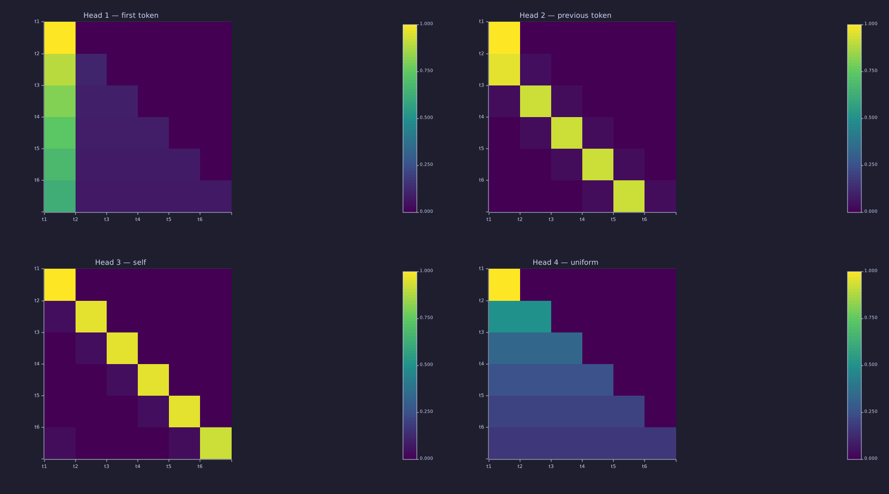
Head 1 lights up column \(t_1\), head 2 the sub-diagonal, head 3 the diagonal, head 4 fills each row's causal triangle evenly. Row 1 of every head is \([1, 0, \dots]\) — with only itself visible, even a "previous-token" head has nowhere else to look. In head 3, row 6 leaks 0.038 onto \(t_1\) as well as \(t_5\): the unit-circle code wraps at \(T = 6\), so position 1 sits next to position 6 — a first taste of the aliasing that Lesson 10 designs around.
All four are lower-triangular (same causal mask) with rows summing to 1 (softmax), yet they compute completely different mixings. Head 4 recovers exactly the uniform prefix average from 07-context-and-naive-averaging — attention is a strict generalisation.
Concatenation and Output Projection
Theory
Per-head outputs \(\mathbf{O}_h \in \mathbb{R}^{T \times d_v}\) are stacked along the feature axis and projected back to \(d_{\text{model}}\):
\[\mathrm{Concat} = [\mathbf{O}_1, \mathbf{O}_2, \dots, \mathbf{O}_H] \in \mathbb{R}^{T \times H d_v}, \qquad \mathbf{O} = \mathrm{Concat} \cdot \mathbf{W}_O.\]
When \(d_v = d_{\text{model}}/H\) the concatenation already has the right shape, but \(\mathbf{W}_O\) is essential: it mixes features across heads so later layers can combine what each head discovered. Without it, slices of \(\mathbf{O}\) come from unrelated heads and the \(H\) parallel computations never interact.
Fan-out on the left (one \(\mathbf{X}\), \(H\) sets of projections), fan-in on the right (\(\mathbf{W}_O\) sums the heads' contributions into one \(d\)-wide stream). The Signals lens below writes this picture as a single equation.
Example — Two-head pipeline with explicit values
The full pipeline in compact form (\(T=4\), \(H=2\), \(d_k=d_v=2\), \(d_{\text{model}}=4\)). With a one-hot \(\mathbf{X} = \mathbf{I}\) the value projections are column slices of \(\mathbf{X}\) — head 1 reads features \(x_3, x_4\) and head 2 reads \(x_1, x_2\), so that both heads have something non-zero to say in the same row — and \(\mathbf{W}_O\) is hand-set to mix the heads: output channel \(d_1\) receives \(h_{1.1} + h_{2.1}\) and channel \(d_3\) receives \(-h_{2.1}\).
T2 = 4;
d_model = 4;
d_k2 = 2;
d_v = 2;
scale2 = 1.0 / sqrt(d_k2);
X = eye(T2);                                % one-hot tokens
M2 = causal_mask(T2);

% Head 1: self-attention on a cyclic position code (as head 3 above)
K1b = zeros(T2, d_k2);
for t = 1:T2
  K1b(t, 1) = 3.0 * cos(2.0 * pi * t / T2);
  K1b(t, 2) = 3.0 * sin(2.0 * pi * t / T2);
end
V1 = X(:, 3:4);                             % W_V^1 selects features x3, x4

% Head 2: uniform over past
Q2b = zeros(T2, d_k2);
K2b = zeros(T2, d_k2);
V2 = X(:, 1:2);                             % W_V^2 selects features x1, x2

A1b = causal_attention_weights(K1b, K1b, scale2, M2);
A2b = causal_attention_weights(Q2b, K2b, scale2, M2);
O1 = A1b * V1;
O2 = A2b * V2;
O_concat = [O1, O2];                        % T × H*d_v

% Output projection: rows = concat columns (h1.1, h1.2, h2.1, h2.2), cols = d1..d4
W_O = [ 1.0, 0.0,  0.0, 0.0;
        0.0, 1.0,  0.0, 0.0;
        1.0, 0.0, -1.0, 0.0;
        0.0, 0.0,  0.0, 1.0 ];
O = O_concat * W_O;

print("Concat = [O_1, O_2]:", O_concat);
print("O = Concat * W_O:", O);
concat_shape = size(O_concat);
out_shape    = size(O);
print("Concat shape =", concat_shape, "   O shape =", out_shape);
n_qkv = 3 * d_model * d_model;
n_wo  = d_model * d_model;
n_tot = n_qkv + n_wo;
print("parameters: W_Q, W_K, W_V =", n_qkv, " W_O =", n_wo, " total =", n_tot);Concat = [O_1, O_2]: Matrix(4x4)
[0.000000, 0.000000, 1.000000, 0.000000]
[0.000000, 0.000000, 0.500000, 0.500000]
[0.998277, 0.000000, 0.333333, 0.333333]
[0.001717, 0.996564, 0.250000, 0.250000]
O = Concat * W_O: Matrix(4x4)
[1.000000, 0.000000, -1.000000, 0.000000]
[0.500000, 0.000000, -0.500000, 0.500000]
[1.331611, 0.000000, -0.333333, 0.333333]
[0.251717, 0.996564, -0.250000, 0.250000]
Concat shape = [1×2] 4.000000 4.000000 O shape = [1×2] 4.000000 4.000000
parameters: W_Q, W_K, W_V = 48 W_O = 16 total = 64Shapes: \(\mathrm{Concat} \in \mathbb{R}^{4 \times 4}\), \(\mathbf{O} \in \mathbb{R}^{4 \times 4}\). Read row 3. Concat holds \([0.998, 0.000, 0.333, 0.333]\) — head 1 put almost all its weight on token 3 itself (feature \(x_3\)), head 2 averaged tokens 1–3 (\(x_1\) and \(x_2\) at \(1/3\) each). In O, channel \(d_1 = h_{1.1} + h_{2.1} = 0.998 + 0.333 = 1.332\): one output channel now carries information from both heads, which no column of Concat did. Channel \(d_3 = -h_{2.1} = -0.333\) is negative, so the heatmap below needs a signed colour scale. A learned \(\mathbf{W}_O\) does the same with dense trained weights instead of hand-set \(\pm 1\).
Example — W_O, Concat and final output heatmaps
Rows of Concat and O are token positions; columns are feature dimensions (\(h_{1.*}\) from head 1, \(h_{2.*}\) from head 2, then \(d_1..d_4\)). \(\mathbf{W}_O\) is drawn with its rows labelled by the concat column it reads and its columns by the output channel it writes.
positions2  = {"t1", "t2", "t3", "t4"};
concat_cols = {"h1.1", "h1.2", "h2.1", "h2.2"};
out_cols    = {"d1", "d2", "d3", "d4"};

figure();
subplot(1, 3, 1)
heatmap(out_cols, concat_cols, W_O, "W_O  (H*d_v × d_model)", "viridis")
subplot(1, 3, 2)
heatmap(concat_cols, positions2, O_concat, "Concat = [O_1, O_2]  (T × H*d_v)", "viridis")
subplot(1, 3, 3)
heatmap(out_cols, positions2, O, "O = Concat * W_O  (T × d_model)", "viridis")
In \(\mathbf{W}_O\) (left), column \(d_1\) has two non-zero rows, \(h_{1.1}\) and \(h_{2.1}\): that is the mixing. Follow it to the right panel — column \(d_1\) of O is the sum of columns \(h_{1.1}\) and \(h_{2.1}\) of Concat — and note the negative column \(d_3\).
Parameter Count
Theory
Pack the per-head projections into three combined \(d_{\text{model}} \times d_{\text{model}}\) matrices; head \(h\) uses columns \((h-1)d_k + 1, \dots, h d_k\). The total is
\[\underbrace{3 d_{\text{model}}^2}_{\mathbf{W}_Q, \mathbf{W}_K, \mathbf{W}_V} + \underbrace{d_{\text{model}}^2}_{\mathbf{W}_O} \;=\; 4 d_{\text{model}}^2.\]
For the toy \(d_{\text{model}} = 4\) that is \(3 \cdot 16 + 16 = 64\) parameters. This counts weight matrices only; a GPT-2-style block also carries \(4 d_{\text{model}}\) bias parameters (one bias per \(\mathbf{Q}, \mathbf{K}, \mathbf{V}, \mathbf{O}\) projection), ignored here as in 11-feed-forward-block.
\(H\) does not appear. More heads at fixed \(d_{\text{model}}\) means narrower heads (\(d_k = d_{\text{model}}/H\)), not more parameters. Head count is an architectural choice; head width is what determines capacity.
Example — The packed W_Q with its head slices
With \(\mathbf{X} = \mathbf{I}\) the projections are the per-head query matrices (\(\mathbf{Q}_h = \mathbf{X}\mathbf{W}_Q^h = \mathbf{W}_Q^h\)), so the packed \(\mathbf{W}_Q\) of the two-head pipeline is simply \([\mathbf{W}_Q^1, \mathbf{W}_Q^2]\): rows are input features, columns are the \(H \cdot d_k = d_{\text{model}}\) query dimensions.
W_Q_packed = [K1b, Q2b];                    % head 1 used Q = K1b; head 2 used Q = 0
Q_all = X * W_Q_packed;                     % one matmul computes every head's Q
slice_err = max(max(abs(Q_all(:, 1:2) - K1b)));
print("max |Q_all(:, 1:2) - Q_1| =", slice_err);

figure();
heatmap({"h1.q1", "h1.q2", "h2.q1", "h2.q2"}, {"x1", "x2", "x3", "x4"}, W_Q_packed, "Packed W_Q (d_model × H*d_k): columns 1–2 = head 1, 3–4 = head 2", "viridis")max |Q_all(:, 1:2) - Q_1| = 0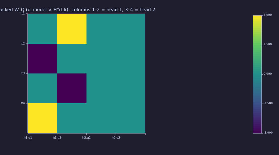
Head 1's slice (columns \(h_{1.q1}, h_{1.q2}\)) is the \(\pm 3\) unit-circle code; head 2's slice is all zeros because the uniform head asks no question. The matrix is \(d_{\text{model}} \times d_{\text{model}}\) however many vertical slices it is cut into — that is why \(H\) drops out of \(4d_{\text{model}}^2\).
Why Does This Work?
Theory
Each head sees the full input \(\mathbf{X}\) but projects it down to a \(d_k\)-dimensional subspace before computing attention. Different projections emphasise different features of \(\mathbf{X}\), so each head sees a different "view" of the sequence. With enough heads and sufficient training, the heads tend to specialise — some learn positional patterns (our heads 2–3), some content patterns (our head 1), some long-range structure. Specialisation is not engineered: because all heads share the same input and loss, training tends to find projections that cover somewhat complementary patterns. The tendency is only partial — head-pruning studies on trained models (e.g. Michel et al., 2019, "Are Sixteen Heads Really Better than One?") remove a large fraction of heads with little loss in quality, so real models carry substantial head redundancy.
Preview — induction heads. The most studied learned pattern combines two of our four heads across two layers. A previous-token head (head 2) in layer 1 writes "the token before me was \(a\)" into each position's residual stream; a head in layer 2 then attends from the current token \(a\) to every earlier position whose predecessor was \(a\) and copies what followed it. The pair implements "the last time I saw \(a\) it was followed by \(b\), so predict \(b\)" — in-context copying, which no single head can express because it needs one head's output as the next head's key. 13-transformer-block stacks the layers that make this possible.
Engineering Lenses
No systems reading adds to this lesson: multi-head attention is a memoryless map from \(\mathbf{X}\) to \(\mathbf{O}\) (its state along time, the key/value cache, appears in 21-sampling-and-generation).
Signals
Exact. Filter bank. Split \(\mathbf{W}_O\) into row blocks \(\mathbf{W}_O^{(h)} \in \mathbb{R}^{d_v \times d_{\text{model}}}\) (rows \((h-1)d_v+1, \dots, h d_v\)). Block matrix multiplication then gives
\[\mathrm{Concat} \cdot \mathbf{W}_O \;=\; \sum_{h=1}^{H} \mathbf{O}_h \mathbf{W}_O^{(h)} \;=\; \sum_{h=1}^{H} \mathbf{A}_h \,\mathbf{X}\, \mathbf{W}_V^h \mathbf{W}_O^{(h)}.\]
Each term is a causal time-varying filter \(\mathbf{A}_h\) along the token axis (Lesson 07's reading of a mixing matrix) composed with a channel map \(\mathbf{W}_V^h \mathbf{W}_O^{(h)}\) of rank at most \(d_v\): \(\mathbf{A}_h\) is the analysis filter, \(\mathbf{W}_O^{(h)}\) the synthesis filter, and MHA is the sum of \(H\) rank-limited filters. This answers both questions at once — \(\mathbf{W}_O\) is there so each head's output lands in the shared \(d_{\text{model}}\)-dimensional stream, and heads "add up" literally.
W_V1 = eye(d_model)(:, 3:4);                % head 1's value projection (selects x3, x4)
W_V2 = eye(d_model)(:, 1:2);                % head 2's value projection (selects x1, x2)
W_O1 = W_O(1:2, :);                         % synthesis block of head 1
W_O2 = W_O(3:4, :);                         % synthesis block of head 2
O_sum = A1b * X * W_V1 * W_O1 + A2b * X * W_V2 * W_O2;
bank_err = max(max(abs(O - O_sum)));
print("max |Concat*W_O - sum_h A_h X W_V^h W_O^(h)| =", bank_err);max |Concat*W_O - sum_h A_h X W_V^h W_O^(h)| = 0The identity holds exactly (maximum deviation 0).
Model. Impulse responses. Row \(t\) of \(\mathbf{A}_h\) is the impulse response seen at output time \(t\). The four heads approach four textbook causal filters as the key gain grows: head 1 a hold on the first sample (a DC hold), head 2 the unit delay \(z^{-1}\), head 3 the identity, head 4 Lesson 07's growing box. At the gain used here the row-4 entropies of \(1.25\) / \(0.47\) / \(0.24\) bits (Information lens below) show heads 1–3 as soft versions of those filters; only head 4 is exact. Attention can realise any causal filter with non-negative taps summing to one — and, unlike a fixed filter, choose the taps per input.
figure();
subplot(1, 4, 1)
stem(1:T, A1(4, :), "color", "blue")
title("head 1: first-sample hold")
xlabel("key position i")
subplot(1, 4, 2)
stem(1:T, A2(4, :), "color", "blue")
title("head 2: unit delay z^-1")
xlabel("key position i")
subplot(1, 4, 3)
stem(1:T, A3(4, :), "color", "blue")
title("head 3: identity")
xlabel("key position i")
subplot(1, 4, 4)
stem(1:T, A4(4, :), "color", "blue")
title("head 4: growing box")
xlabel("key position i")
Each panel is row 4 of one head — the taps applied to keys \(1..6\) when the query sits at \(t = 4\). Taps at \(i > 4\) are exactly zero (causal); the non-zero taps sum to one (softmax).
Exact. Rank. \(\mathbf{Q}_h\mathbf{K}_h^\top\) is \(T \times T\) but factors through \(d_k = 2\) columns, so its rank is at most 2. Head 1's score matrix has rank 1 (a single key feature), head 4's has rank 0 (all scores zero); heads 2–3 use the full budget. \(H\) narrow heads therefore give \(H\) independent rank-\(d_k\) score matrices where one wide head gives a single rank-\(d_{\text{model}}\) one — at identical cost:
print("rank(Q_h K_h') for heads 1..4:", rank(Q1 * K1'), rank(Q2 * K2'), rank(K2 * K2'), rank(Q4 * K4'));
T_big = 1024;
d_big = 512;
H_big = 8;
flops_wide   = 2 * T_big^2 * d_big;                    % one head of width d
flops_narrow = H_big * 2 * T_big^2 * (d_big / H_big);  % H heads of width d/H
print("score FLOPs, one wide head vs H narrow heads:", flops_wide, flops_narrow);rank(Q_h K_h') for heads 1..4: 1 2 2 0
score FLOPs, one wide head vs H narrow heads: 1073741824 1073741824Information
Exact. Selectivity in bits. The row entropy \(H(\mathbf{A}_h[t,:])\) (Lesson 08) measures how many past positions a head effectively blends at query \(t\); the ceiling is \(\log_2 t\) bits (uniform). Computed on the four heads above:
Hs = [row_entropies_bits(A1)', row_entropies_bits(A2)', row_entropies_bits(A3)', row_entropies_bits(A4)'];
Htab = [(1:T)', log2(1:T)', Hs];
print("columns: t, log2 t, head 1, head 2, head 3, head 4  (bits)");
print(Htab);columns: t, log2 t, head 1, head 2, head 3, head 4 (bits)
Matrix(6x6)
[1.000000, 0.000000, 0.000000, 0.000000, 0.000000, 0.000000]
[2.000000, 1.000000, 0.490928, 0.241602, 0.241602, 1.000000]
[3.000000, 1.584963, 0.901880, 0.466890, 0.242633, 1.584963]
[4.000000, 2.000000, 1.252685, 0.467871, 0.242689, 2.000000]
[5.000000, 2.321928, 1.556962, 0.467924, 0.243721, 2.321928]
[6.000000, 2.584963, 1.824399, 0.468905, 0.468905, 2.584963]| \(t\) | \(\log_2 t\) | head 1 (first) | head 2 (previous) | head 3 (self) | head 4 (uniform) |
|---|---|---|---|---|---|
| 2 | 1.00 | 0.49 | 0.24 | 0.24 | 1.00 |
| 4 | 2.00 | 1.25 | 0.47 | 0.24 | 2.00 |
| 6 | 2.58 | 1.82 | 0.47 | 0.47 | 2.58 |
Head 4 sits exactly on the ceiling — it selects nothing. Heads 2 and 3 spend 0.47 and 0.24 bits at \(t = 4\), i.e. \(2^{H}\) ≈ 1.38 and 1.18 effective positions — nearly one-hot. Head 1 is the softest: its score margin of \(3/\sqrt{2}\) leaves 1.82 bits at \(t = 6\) (about 3.5 effective positions), so a sharper "first token" head needs a larger key magnitude (Exercise 6).
Model. Joint versus per-head information. Each head extracts a fragment of the mutual information \(I(X_{t+1}; X_{1..t})\) that Lesson 08 identified as attention's prediction signal. Two heads that recover the same fragment are redundant — \(I(X_{t+1}; \mathbf{o}_t^{(h_1)}, \mathbf{o}_t^{(h_2)})\) equals either head's individual contribution — while heads recovering different fragments add. Cross-entropy training therefore rewards complementary heads, but only weakly: the pruning results above show trained models keep many near-redundant heads. Heads 2 and 3 here are an example — both are pure position and, past \(t = 2\), carry the same information about where to look. \(\mathbf{W}_O\) then re-mixes the surviving fragments into one dense representation for the next layer.
Key Takeaways
- Why multiple heads: one softmax gives one convex combination per position and a rank-\(\le d_k\) score matrix; \(H\) heads give \(H\) simultaneous retrievals at the FLOPs of one wide head.
- Per-head: run Lesson-08 attention with its own \(\mathbf{W}_Q^h, \mathbf{W}_K^h, \mathbf{W}_V^h\).
- Concat + project: stack head outputs along the feature axis, then project with \(\mathbf{W}_O\) to mix them; equivalently, \(\mathrm{Concat}\cdot\mathbf{W}_O = \sum_h \mathbf{A}_h\mathbf{X}\mathbf{W}_V^h\mathbf{W}_O^{(h)}\) — a filter bank whose synthesis filters are the row blocks of \(\mathbf{W}_O\).
- Four heads, four filters: first-sample hold, unit delay \(z^{-1}\), identity, growing box; their row entropies (≈ 0.5, ≈ 0.25 and \(\log_2 t\) bits) measure how selective each is.
- Parameter count: \(4 d_{\text{model}}^2\) — independent of the number of heads when \(d_k = d_{\text{model}}/H\).
- Uniform averaging (Lesson 07) is a special case: a degenerate head with zero \(\mathbf{Q}\) and \(\mathbf{K}\) produces exactly the prefix-average matrix.
Standalone Scripts
| Script | What it computes |
|---|---|
multi_head_weights.rlab | four hand-crafted heads (first-token, previous-token, self, uniform) as one 2×2 heatmap grid; ranks of the score matrices; per-row entropies in bits; the row-4 impulse responses |
head_concatenation.rlab | full \(T=4, H=2\) pipeline: per-head \(\mathbf{O}_h\) via column slices, concat, the mixing \(\mathbf{W}_O\) (signed heatmaps); the packed \(\mathbf{W}_Q\); parameter count |
filter_bank_identity.rlab | verifies \(\mathrm{Concat}\cdot\mathbf{W}_O = \sum_h \mathbf{A}_h\mathbf{X}\mathbf{W}_V^h\mathbf{W}_O^{(h)}\) for the mixing, identity and permutation \(\mathbf{W}_O\); one-wide-head vs \(H\)-narrow-head FLOPs |
Run all with make lesson-09 (or rustlab run lessons/09-multi-head-attention/<name>.rlab).
Expected Numerical Outputs Summary
| Variable | Expected Value |
|---|---|
A4_row4 | [0.25, 0.25, 0.25, 0.25, 0, 0] (uniform over past) |
Each row of A1, A2, A3, A4 | sums to 1.0 |
O_concat(3, :) | [0.998, 0, 0.333, 0.333] |
O(3, :) | [1.332, 0, -0.333, 0.333] (\(d_1 = h_{1.1} + h_{2.1}\), \(d_3 = -h_{2.1}\)) |
concat_shape, out_shape | [4, 4] (T × H*d_v and T × d_model) |
slice_err | 0 (the packed \(\mathbf{W}_Q\) slice reproduces \(\mathbf{Q}_1\)) |
n_qkv, n_wo, n_tot | 48, 16, 64 (= \(4 d_{\text{model}}^2\)) |
bank_err | 0 (filter-bank identity) |
rank(Q_h K_h') for heads 1–4 | 1, 2, 2, 0 (all \(\le d_k = 2\)) |
flops_wide, flops_narrow | both 1073741824 |
Hs(4, :) (row-4 entropies, bits) | [1.25, 0.47, 0.24, 2.00] |
Hs(6, :) | [1.82, 0.47, 0.47, 2.58] |
Exercises
- Role of \(\mathbf{W}_O\). In
head_concatenation.rlabreplace the mixing \(\mathbf{W}_O\) first with \(\mathbf{I}\) and then with the permutation that swaps the two head blocks. In which case does any output channel depend on more than one head? Argue why a learned \(\mathbf{W}_O\) is important even though the concatenation already has the correct shape. - Varying \(H\) at fixed \(d_{\text{model}}\). For \(d_{\text{model}} = 384\), compute \(d_k\) and the total parameter count for \(H \in \{1, 2, 4, 6, 8, 12\}\). Confirm the parameter count is independent of \(H\). What trades off as \(H\) grows?
- More heads, same roles. Extend
multi_head_weights.rlabto 8 heads, with heads 5–8 replicating heads 1–4. Do the outputs still differ (they see the same \(\mathbf{V}\))? What does this suggest about initialisation and training? - Attending to two things at once. Design a pair of \((\mathbf{Q}_h, \mathbf{K}_h)\) values so that attention row 4 concentrates roughly evenly on positions 1 and 3 but not 2 or 4. What property of softmax makes this possible, and what does it cost in row entropy compared with a one-hot head?
- Head count vs. dimension budget. A model with \(d_{\text{model}} = 512\) and \(H = 8\) has \(d_k = 64\). If you kept \(d_k\) fixed at 64 but grew \(H\) to 16, how would the parameter count change? Why do practitioners typically fix \(d_k\) (not \(H\)) when scaling model width?
- A sharper first-token head. Scale
K1(1, 1)from 3 to 6 and to 9 and recomputerow_entropies_bits(A1). How many bits does head 1 spend at \(t = 6\) in each case, and what key magnitude brings its effective position count \(2^{H}\) below 1.1?
What's next
This completes the attention mechanism. Phase 4 (Lessons 10–12) builds the three supporting pieces that surround attention in a transformer block: 10-positional-encoding (so the model knows where each token sits — attention itself is order-blind, as heads 2–3 above had to be told by hand), the MLP feed-forward sublayer (per-position non-linearity), and LayerNorm with residual connections (the stabilisers that let many blocks stack deep without exploding or vanishing).