Lesson 17: Learning Rate Scheduling
16-adamw-optimizer treated the learning rate \(\eta\) as a single fixed number. Real LLM training never holds \(\eta\) constant. Instead it follows a schedule: a short linear warmup at the start, then a long cosine decay. In control terms a schedule is gain scheduling — the loop gain of the training controller is moved along a planned trajectory during the run. This lesson derives the warmup-then-cosine schedule used in nanoGPT, GPT-3, LLaMA, and most modern transformers, shows what a time-varying gain does to each mode of the loss, and shows why the decay is what finally removes the optimiser's noise floor.
Learning Objectives
- Define linear warmup and give the reasons a transformer needs a small learning rate at the start — Adam's sign-sized first step first among them.
- Define cosine decay with a minimum-LR floor and explain why it converges more smoothly than step decay or exponential decay.
- Combine the two into a single \(\eta(t)\) function and plot it.
- Read a schedule as a linear time-varying system: the per-mode contraction factor \(\lvert 1 - \eta_t\lambda_i \rvert\), its running product, and the noise floor \(\propto \eta\).
- Recognise the hyperparameters that real LLM training papers report:
warmup_steps,lr_decay_steps,min_lr,max_lr.
Background
Adam and AdamW from 16-adamw-optimizer, including the stability bound \(\eta < 2/\lambda_{\max}\) (one mode there; the matrix version in 06-linear-layers-and-gradient-descent) and the one-pole-filter reading of the moments. Cross-entropy loss as the optimisation target from 03-cross-entropy-loss.
The Warmup Phase
Theory
Warmup ramps \(\eta\) linearly from 0 to \(\eta_{\max}\) over the first \(T_w\) steps:
\[\eta_{\text{warmup}}(t) \;=\; \eta_{\max} \cdot \frac{t}{T_w} \quad \text{for } t \in [0, T_w].\]
The cleanest reason it is needed is two lines of arithmetic. At \(t = 1\) Adam's bias-corrected moments are \(\hat{\mathbf{m}}_1 = \mathbf{g}_1\) and \(\hat{\mathbf{v}}_1 = \mathbf{g}_1^2\) exactly, so
\[\frac{\hat{\mathbf{m}}_1}{\sqrt{\hat{\mathbf{v}}_1}} = \frac{\mathbf{g}_1}{\lvert \mathbf{g}_1 \rvert} = \operatorname{sign}(\mathbf{g}_1).\]
The first update moves every parameter by exactly \(\eta_1\), whatever the size of its gradient: a coordinate with gradient \(10^{-3}\) and one with gradient \(300\) take the same step. At \(\eta_1 = \eta_{\max}\) that is a full-sized, effectively random-signed kick to all \(N\) parameters at once — a displacement of \(\eta_{\max}\sqrt{N}\) — before \(\hat{\mathbf{v}}\) carries any information about scale. Warmup makes the first kick \(\eta_{\max}/T_w\) instead, and for the next few dozen steps, while \(\hat{\mathbf{v}}\) is still an average over only \(t\) samples, keeps the steps small while the scale estimate settles.
That is one reason among several, which is why how long to warm up is set empirically rather than by a formula: the loss surface at initialisation is unusually sharp along a few directions (its \(\lambda_{\max}\) is large, so the stable \(\eta\) is small until the first steps flatten it); embedding rows of tokens not yet seen have \(\hat v = 0\) and take full-sized steps the moment they first appear; and Post-LN transformer stacks are unstable without warmup (Xiong et al., 2020 — the reason 12-layer-norm-and-residuals moved to Pre-LN). Published values: GPT-3 warms up over its first 375 M tokens, LLaMA-1 and LLaMA-2 use 2000 steps, small char-level runs use 100–500. Adam's second-moment horizon \(1/(1-\beta_2)\) is not the anchor: LLM practice uses \(\beta_2 = 0.95\) (a 20-step horizon, 16-adamw-optimizer) with warmups of thousands of steps.
Example — Adam's first step is sign(g)
beta1 = 0.9;  beta2 = 0.999;
g1 = [0.001, -300.0, 4.0];                    % three coordinates, gradients 5 orders apart
m_hat1 = ((1 - beta1) * g1) / (1 - beta1);
v_hat1 = ((1 - beta2) * g1 .^ 2) / (1 - beta2);
kick = 6e-4 * sqrt(124e6);                    % GPT-2 124M at eta_max = 6e-4, no warmup
print("g_1                    :", g1);
print("m_hat_1 ./ sqrt(v_hat_1):", m_hat1 ./ sqrt(v_hat1));
print("un-warmed first step, GPT-2 124M: ||step|| = eta_max sqrt(N) =", kick, " (init norm 0.02 sqrt(N) =", 0.02 * sqrt(124e6), ")");g_1 : [1×3] 0.001000 -300.000000 4.000000
m_hat_1 ./ sqrt(v_hat_1): [1×3] 1.000000 -1.000000 1.000000
un-warmed first step, GPT-2 124M: ||step|| = eta_max sqrt(N) = 6.681317235396026 (init norm 0.02 sqrt(N) = 222.7105745132009 )Every coordinate reports \(\pm 1\): at step one Adam is sign descent, and \(\eta_1\) alone sets the step size. For a 124 M-parameter GPT-2 at \(\eta_{\max} = 6\times10^{-4}\) the un-warmed first step would move the whole parameter vector by \(6.7\) in Euclidean norm — about 3 % of the initialisation's norm, in one step, in a direction chosen by a single minibatch.
The Cosine Decay Phase
Theory
After warmup, decay \(\eta\) smoothly from \(\eta_{\max}\) down to a floor \(\eta_{\min}\) over the remaining \(T_d - T_w\) steps:
\[\eta_{\text{decay}}(t) \;=\; \eta_{\min} + \tfrac{1}{2}(\eta_{\max} - \eta_{\min})\left(1 + \cos\!\left(\pi \cdot \frac{t - T_w}{T_d - T_w}\right)\right)\quad \text{for } t \in (T_w, T_d].\]
At \(t = T_w\) this evaluates to \(\eta_{\max}\) (the cosine is \(\cos 0 = 1\)); at \(t = T_d\) it evaluates to \(\eta_{\min}\) (the cosine is \(\cos \pi = -1\)). The shape is slow-fast-slow: gentle decrease at the start of the decay (so we keep exploring near the still-high LR), aggressive drop in the middle, gentle approach to the floor near the end (so the final updates are small enough to settle into a flat region of the loss surface).
Why cosine and not exponential or step decay?
- Step decay (drop by 10× at fixed milestones) introduces sudden gradient-magnitude shocks that disrupt Adam's moment estimates.
- Exponential decay \(\eta_t = \eta_0 \gamma^t\) is too aggressive early and too slow late.
- Cosine has zero derivative at both ends of the decay segment — it leaves the peak flat and approaches the floor flat, so the late-training LR settles gently instead of dropping in shocks the way step decay does. (The composite schedule does have one slope kink at \(t = T_w\), where the warmup ramp of slope \(\eta_{\max}/T_w\) meets the decay's zero slope. That single kink at the peak is harmless; step decay introduces a fresh one at every milestone.)
A typical schedule sets \(\eta_{\min} = 0.1 \cdot \eta_{\max}\). The 10× cap on the LR range keeps the optimiser productive even at the end of training. Two relatives you will meet in current papers: warmup–stable–decay (WSD) holds \(\eta_{\max}\) flat for most of the run and decays only in a short final cooldown, so the total run length need not be fixed in advance; and the original Transformer's inverse-square-root schedule, \(\eta_t \propto \min\!\big(t^{-1/2},\, t\,T_w^{-3/2}\big)\), decays forever without a floor.
Example — Build the full schedule and plot it
T_total  = 5000;
T_warmup = 500;
T_decay  = T_total;
eta_max  = 6e-4;
eta_min  = 6e-5;

eta_sched = zeros(T_total + 1);
for t = 0:T_total
  if t < T_warmup
    eta_sched(t + 1) = eta_max * (t / T_warmup);
  else
    progress = (t - T_warmup) / (T_decay - T_warmup);
    eta_sched(t + 1) = eta_min + 0.5 * (eta_max - eta_min) * (1 + cos(pi * progress));
  end
endfigure();
steps = 0:T_total;
plot(steps, eta_sched, "color", "blue", "label", "warmup + cosine")
title("Learning-rate schedule (T_w=500, T_total=5000)")
xlabel("step")
ylabel("eta")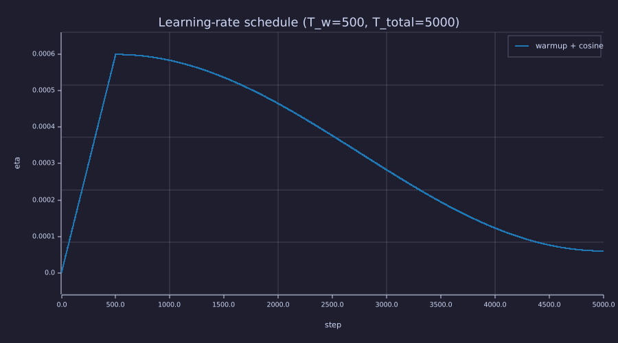
Three regions: a steep linear ramp to the peak in the first 500 steps, a flat shoulder near the peak (zero slope where the cosine starts), and a long decay that flattens again into the floor at \(6\times10^{-5}\).
Schedule and Loss Curve
Theory
On a quadratic, gradient descent with a constant \(\eta\) is linear time-invariant: along each eigen-direction of the Hessian with curvature \(\lambda_i\) the error obeys \(e_{t+1} = (1 - \eta\lambda_i)\,e_t\) — the pole of 16-adamw-optimizer — and is stable iff \(\lvert 1 - \eta\lambda_i \rvert < 1\). A schedule makes the same system linear time-varying: the pole moves every step, and
\[e_t = \Big(\prod_{s=1}^{t} (1 - \eta_s\lambda_i)\Big)\, e_0 .\]
What matters per mode is therefore the contraction factor \(\lvert 1 - \eta_t\lambda_i \rvert\) at each step and its running product. A factor above 1 for a few steps is harmless; a factor above 1 forever is divergence; a factor of exactly 0 (at \(\eta_t = 1/\lambda_i\)) annihilates that mode's error in a single step. This is gain scheduling in the textbook sense: \(\eta_t\) is planned so that the fast modes are never held above 1, most of the run is spent near the largest safe gain, and — once gradient noise is included — the noise floor, which scales with \(\eta\), is lowered at the end. The honest comparison with a constant learning rate is then not "the schedule wins on final loss" (a patient constant-low run reaches the same floor) but "the schedule keeps every mode contracting while getting to the floor several times sooner, and never risks the divergence the high-gain run suffers".
Example — Three runs through one helper
A noisy quadratic surrogate with curvature 10 in \(\theta_1\) and 1 in \(\theta_2\), so the fast mode's stability limit is \(\eta < 2/10 = 0.2\). One helper, run_sgd, takes the schedule as a function of \(t\) and returns the loss curve, the \(\eta_t\) actually used, and the per-step gradient signal-to-noise ratio (used under the Information lens). Three calls: a constant \(\eta = 0.25\) above the limit, a constant \(\eta = 0.02\) well below it, and warmup + cosine (peak \(0.18\), floor \(0.02\)).
seed(17);
function L = surrogate_loss(theta)
  L = 0.5 * (10.0 * theta(1) ^ 2 + theta(2) ^ 2) + 1.0;   % +1 floor like real CE
end
function g = surrogate_grad(theta)
  g = [10.0 * theta(1), theta(2)];
end
function e = warmup_cosine(t, T_w, T_d, eta_p, eta_f)
  if t <= T_w
    e = eta_p * (t / T_w);
  else
    e = eta_f + 0.5 * (eta_p - eta_f) * (1 + cos(pi * (t - T_w) / (T_d - T_w)));
  end
end
% One noisy-SGD run under the schedule eta_of_t(t).  Returns the loss curve,
% the eta_t actually used, and the per-step SNR  ||grad L||^2 / (2 sigma^2).
function [L, etas, snr] = run_sgd(eta_of_t, n, sigma, init)
  theta = init;  L = zeros(n + 1);  etas = zeros(n);  snr = zeros(n);
  L(1) = surrogate_loss(theta);
  for t = 1:n
    etas(t) = eta_of_t(t);
    g_true = surrogate_grad(theta);
    snr(t) = sum(g_true .^ 2) / (2 * sigma ^ 2);
    theta = theta - etas(t) * (g_true + sigma * randn(2));
    L(t + 1) = surrogate_loss(theta);
  end
end

n_train = 300;  sigma = 0.3;  init = [-3.0, 2.0];
T_w = 30;  eta_p = 0.18;  eta_f = 0.02;
[loss_high,  eta_high, snr_high]  = run_sgd(@(t) 0.25, n_train, sigma, init);
[loss_low,   eta_low,  snr_low]   = run_sgd(@(t) 0.02, n_train, sigma, init);
[loss_sched, eta_run,  snr_sched] = run_sgd(@(t) warmup_cosine(t, T_w, n_train, eta_p, eta_f), n_train, sigma, init);
print("constant high LR (0.25) final loss:", loss_high(n_train + 1), " (diverged)");
print("constant low  LR (0.02) final loss:", loss_low(n_train + 1));
print("warmup+cosine final loss:", loss_sched(n_train + 1));constant high LR (0.25) final loss: 196059472798838970000000000000000000000000000000000000000000000000000000000000000000000000000000000000000000 (diverged)
constant low LR (0.02) final loss: 1.0006252375809246
warmup+cosine final loss: 1.0018362245113204thresh = 1.01; N = n_train + 1; % loss < 1.01 = "arrived at the floor"
i = 1;
while i < N && loss_low(i) >= thresh
i = i + 1;
end
step_low = i - 1; % curve index k holds step k-1
i = 1;
while i < N && loss_sched(i) >= thresh
i = i + 1;
end
step_sched = i - 1;
i = 1;
while i < N && loss_high(i) <= 1.0e4
i = i + 1;
end
exit_step = i - 1;
print("steps to loss < 1.01 (constant low) :", step_low);
print("steps to loss < 1.01 (warmup+cosine):", step_sched, " ratio", step_low / step_sched);
print("constant-high loss passes 1e4 at step:", exit_step);Steps to reach the floor, and where the diverging run leaves the plot
steps to loss < 1.01  (constant low) : 127
steps to loss < 1.01  (warmup+cosine): 36    ratio 3.5277777777777777
constant-high loss passes 1e4 at step: 7
Example — The contraction factor of each mode
The central figure of this lesson: \(\lvert 1 - \eta_t\lambda \rvert\) for the fast mode (\(\lambda = 10\)) and the slow mode (\(\lambda = 1\)) under the three schedules, against the line at 1.
t_ax = 1:n_train;
lam_fast = 10.0;  lam_slow = 1.0;
figure();
subplot(1, 2, 1)
plot(t_ax, abs(1 - eta_high * lam_fast), "color", "red",   "label", "constant 0.25")
hold("on")
plot(t_ax, abs(1 - eta_low * lam_fast),  "color", "blue",  "label", "constant 0.02")
plot(t_ax, abs(1 - eta_run * lam_fast),  "color", "green", "label", "warmup + cosine")
hline(1, "gray", "stability limit")
hold("off")
title("fast mode: |1 - 10 eta_t|")
xlabel("step")
ylabel("contraction factor")
legend("0.25", "0.02", "schedule", "= 1")
subplot(1, 2, 2)
plot(t_ax, abs(1 - eta_high * lam_slow), "color", "red",   "label", "constant 0.25")
hold("on")
plot(t_ax, abs(1 - eta_low * lam_slow),  "color", "blue",  "label", "constant 0.02")
plot(t_ax, abs(1 - eta_run * lam_slow),  "color", "green", "label", "warmup + cosine")
hline(1, "gray", "stability limit")
hold("off")
title("slow mode: |1 - eta_t|")
xlabel("step")
ylabel("contraction factor")
legend("0.25", "0.02", "schedule", "= 1")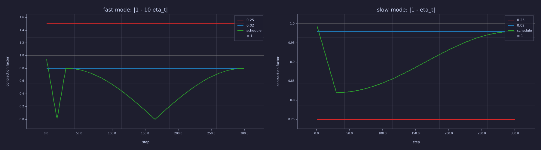
Left: the red run sits at \(1.5\) — above the line — for every step: that is the divergence. The green run starts at \(0.94\) (\(\eta_1 = 0.006\)), dips to \(0.02\) at step 17 on the way up and to exactly \(0\) at step 165 on the way down — both where \(\eta_t \approx 1/\lambda = 0.1\), deadbeat for this mode — and never exceeds \(0.8\). Right: for the slow mode every run is below 1 — even \(\eta = 0.25\) would have been fine for this mode alone (\(0.75\)); the slow run's \(0.98\) is why it takes 127 steps.
Example — Loss curves on a log axis
figure();
steps = 0:n_train;
semilogy(steps, loss_high,  "color", "red",   "label", "constant 0.25")
hold("on")
semilogy(steps, loss_low,   "color", "blue",  "label", "constant 0.02")
semilogy(steps, loss_sched, "color", "green", "label", "warmup + cosine")
hline(1.01, "gray", "floor + 1 %")
hold("off")
ylim([0.9, 1.0e4])
title("loss under three LR strategies (log axis, frame cropped at 1e4)")
xlabel("step")
ylabel("L")
legend("0.25", "0.02", "schedule", "1.01")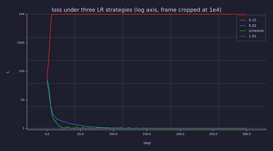
The red curve leaves the top of the frame at step 7: nothing is clamped, the axis is simply cropped at \(10^4\). The green curve crosses the floor line at step 36 and the blue one at step 127.
With \(\eta = 0.25\) the fast mode's factor is \(1.5\) per step, so the loss (quadratic in the error) grows by \(2.25\times\) per step and reaches \(2.0e+107\) by step 300. The low-LR run descends smoothly but only reaches the floor around step \(127\); the schedule reaches the same floor around step \(36\) — about 3.5× sooner — by spending its middle phase near the peak gain. Neither converged run "wins" on final loss (both land at ≈ 1.001, and both end at \(\eta = 0.02\), so they share the same noise floor — see the Signals lens); the schedule simply gets there faster while the high-LR run never gets there at all.
Hyperparameter Cheat Sheet
Theory
What real published transformers use:
| Model | \(\eta_{\max}\) | \(T_w\) | \(T_d\) | \(\eta_{\min} / \eta_{\max}\) |
|---|---|---|---|---|
| nanoGPT GPT-2 124M repro | \(6 \times 10^{-4}\) | 2000 | 600000 | 0.1 |
| GPT-3 (175B) | \(6 \times 10^{-5}\) | 375 M tokens | 260 B tokens | 0.1 |
| LLaMA-1 (7B) | \(3 \times 10^{-4}\) | 2000 | 1 T tokens | 0.1 |
| LLaMA-2 (70B) | \(1.5 \times 10^{-4}\) | 2000 | 2 T tokens | 0.1 |
Patterns to notice:
- \(\eta_{\max}\) decreases sublinearly with model size — bigger models need smaller peak LRs because they have more parameters whose collective updates can destabilise the loss (a 1400× jump from 124 M to 175 B params drops \(\eta_{\max}\) only 10×).
- \(T_w\) stays in the hundreds-to-thousands range and is only weakly dependent on model size. It is an empirical setting — long enough for the early sharpness to relax and for every embedding row to have been touched — not a quantity derived from \(\beta_2\).
- \(\eta_{\min} / \eta_{\max} \approx 0.1\) is the universal default. Going lower wastes the tail of training; going higher leaves Adam too jittery to settle.
Engineering Lenses
Signals
Exact. For the quadratic model, gradient noise enters each mode's recursion as \(e_{t+1} = (1 - \eta\lambda)\,e_t - \eta\,\xi_t\) with \(\xi_t\) white of variance \(\sigma^2\) — a one-pole filter driven by white noise. Its steady-state output variance is
\[\operatorname{Var}\,e = \frac{\eta^2\sigma^2}{1 - (1 - \eta\lambda)^2} = \frac{\eta\,\sigma^2}{\lambda\,(2 - \eta\lambda)}, \qquad \text{excess loss per mode } \tfrac{1}{2}\lambda\,\operatorname{Var}\,e = \frac{\eta\,\sigma^2}{2\,(2 - \eta\lambda)}.\]
The noise floor is proportional to \(\eta\) (until \(\eta\lambda\) approaches 2, where the denominator collapses). That is what the decay buys: a run that ends at \(\eta_{\min} = \eta_{\max}/10\) ends with a floor ten times lower than it had at the peak. Check it by sweeping a constant \(\eta\) and measuring the mean excess loss over the second half of a long run:
seed(171);
etas_sw = logspace(-2, log10(0.19), 6);
meas = zeros(6);  pred = zeros(6);
for i = 1:6
  e = etas_sw(i);
  [Lc, ec, sc] = run_sgd(@(t) e, 4000, sigma, init);
  meas(i) = mean(Lc(2002:4001)) - 1.0;
  pred(i) = e * sigma ^ 2 / (2 * (2 - e * lam_fast)) + e * sigma ^ 2 / (2 * (2 - e * lam_slow));
end
figure();
loglog(etas_sw, pred, "color", "gray",  "label", "theory")
hold("on")
loglog(etas_sw, meas, "color", "green", "label", "measured")
hold("off")
title("steady-state excess loss vs constant eta (sigma = 0.3)")
xlabel("eta")
ylabel("E[L] - 1")
legend("sum over modes of eta sigma^2 / (2 (2 - eta lambda))", "measured, steps 2001-4000")
print("eta      :", etas_sw);
print("measured :", meas);
print("predicted:", pred);eta : [1×6] 0.010000 0.018020 0.032471 0.058513 0.105439 0.190000
measured : [1×6] 0.000477 0.000740 0.001554 0.003433 0.008106 0.083488
predicted: [1×6] 0.000463 0.000855 0.001615 0.003217 0.007522 0.090224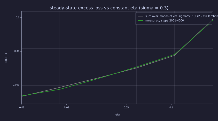
Slope \(+1\) on log–log axes — the floor is linear in \(\eta\) — with the upturn at the right end as \(\eta\) approaches the fast mode's limit \(0.2\). The measured points follow the formula with no fitted constant.
Systems
Exact. Per mode the state is the error \(e_t\) along that eigen-direction, the update law is \(e_{t+1} = (1 - \eta_t\lambda_i)\,e_t\), and the total gain after \(t\) steps is the running product of the contraction factors plotted above. The product is what decides convergence, so plot its logarithm: the constant-high run's fast mode climbs by \(\log_{10} 1.5\) per step, the constant-low run's slow mode falls by only \(\log_{10} 0.98\), and the schedule's fast mode passes through the deadbeat zero (clipped at \(10^{-12}\) per step so the log axis survives).
E3 = [eta_high; eta_low; eta_run];                       % 3 x n_train
P_fast = zeros(3, n_train);  P_slow = zeros(3, n_train);
for r = 1:3
  P_fast(r, :) = cumsum(log10(max(abs(1 - E3(r, :) * lam_fast), 1e-12)));
  P_slow(r, :) = cumsum(log10(abs(1 - E3(r, :) * lam_slow)));
end
figure();
subplot(1, 2, 1)
plot(t_ax, P_fast(1, :), "color", "red",   "label", "constant 0.25")
hold("on")
plot(t_ax, P_fast(2, :), "color", "blue",  "label", "constant 0.02")
plot(t_ax, P_fast(3, :), "color", "green", "label", "warmup + cosine")
hold("off")
title("fast mode: log10 of the running gain")
xlabel("step")
ylabel("log10 |e_t / e_0|")
legend("0.25", "0.02", "schedule")
subplot(1, 2, 2)
plot(t_ax, P_slow(1, :), "color", "red",   "label", "constant 0.25")
hold("on")
plot(t_ax, P_slow(2, :), "color", "blue",  "label", "constant 0.02")
plot(t_ax, P_slow(3, :), "color", "green", "label", "warmup + cosine")
hold("off")
title("slow mode: log10 of the running gain")
xlabel("step")
ylabel("log10 |e_t / e_0|")
legend("0.25", "0.02", "schedule")
print("log10 gain after 300 steps, fast mode (0.25 / 0.02 / schedule):", P_fast(1, n_train), P_fast(2, n_train), P_fast(3, n_train));
print("log10 gain after 300 steps, slow mode (0.25 / 0.02 / schedule):", P_slow(1, n_train), P_slow(2, n_train), P_slow(3, n_train));log10 gain after 300 steps, fast mode (0.25 / 0.02 / schedule): 52.8273777167044 -29.073003902416875 -130.74047586714738
log10 gain after 300 steps, slow mode (0.25 / 0.02 / schedule): -37.48162098248998 -2.632177292251555 -13.841331073768968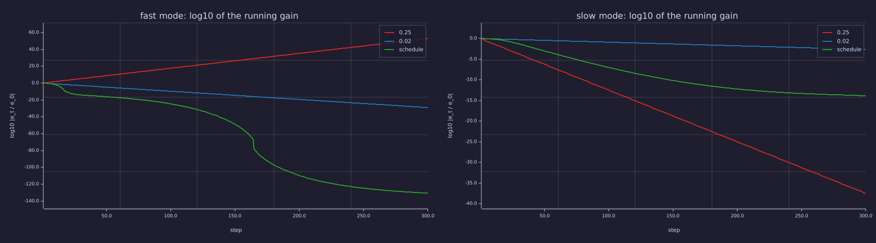
Left: red rises by 53 decades — the noiseless fast mode of the \(\eta = 0.25\) run would be \(10^{53}\) times its starting error. Right: the slow mode is where the constant-low run loses — \(0.98^{300}\) is only \(2.6\) decades, while the schedule buys \(14\).
Analogy. Warmup is often called a soft start, after the ramped supply that limits inrush current while a motor's state is still unknown. The picture is right about why (limit the first kick while the plant state — the loss surface's local curvature and \(\hat{\mathbf{v}}\) — is unknown) but it is only a picture: there is no current, no flux, and no conserved quantity being protected. The exact content is the contraction factor above and the sign-descent first step at the top of the lesson.
Information
Model. The gradient is a noisy channel carrying the descent direction. Per step its signal-to-noise ratio is \(\mathrm{SNR}_t = \lVert \nabla L(\theta_t) \rVert^2 / (2\sigma^2)\) — run_sgd records it — and by the Gaussian-channel bound a step can convey at most \(\tfrac{1}{2}\log_2(1 + \mathrm{SNR}_t)\) bits about that direction. Early in the run the gradient is large and the channel is clean; near the floor the true gradient is a small fraction of the noise and each step carries a fraction of a bit. A schedule matches the step size to that budget: large steps while the gradient is informative, small ones when it is mostly noise (and, by the Signals lens, the small steps are also what keep the noise-driven wander small).
bits = @(s) 0.5 * log2(1 + s);
figure();
semilogy(t_ax, snr_low,   "color", "blue",  "label", "constant 0.02")
hold("on")
semilogy(t_ax, snr_sched, "color", "green", "label", "warmup + cosine")
hline(1, "gray", "SNR = 1")
hold("off")
title("per-step gradient SNR  ||grad L||^2 / (2 sigma^2)")
xlabel("step")
ylabel("SNR")
legend("0.02", "schedule", "SNR = 1")
snr_end_low = mean(snr_low(271:300));  snr_end_sched = mean(snr_sched(271:300));
print("SNR at step 1:", snr_sched(1), "  ->", bits(snr_sched(1)), "bits/step");
print("SNR, mean of steps 271-300:  low", snr_end_low, "  schedule", snr_end_sched);
print("bits/step at the end : low", bits(snr_end_low), " schedule", bits(snr_end_sched));SNR at step 1: 5022.222222222223 -> 6.147198692219589 bits/step
SNR, mean of steps 271-300: low 0.04033768319248866 schedule 0.08986671853904973
bits/step at the end : low 0.028525944372010593 schedule 0.06207585820767956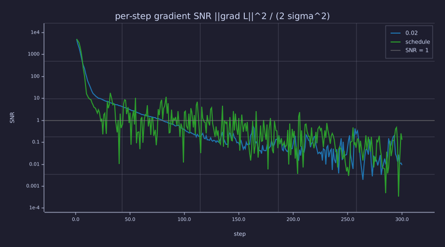
Both runs start near \(\mathrm{SNR} = 5022\) and end below the line; the schedule reaches the noise-dominated regime by step ≈ 40 and then, correctly, takes small steps for the remaining 260.
At step 1 the channel carries \(6.1\) bits per step; over the last 30 steps the SNR averages \(0.09\) for the scheduled run — \(0.06\) bits per step — the regime where only small steps make sense. Read this way an LR schedule is not a heuristic: it is a time-varying step size matched to the information the gradient currently carries.
Key Takeaways
- Warmup ramps \(\eta\) from 0 to \(\eta_{\max}\) over the first hundreds-to-thousands of steps. Adam's first step is exactly \(\eta_1\,\operatorname{sign}(\mathbf{g}_1)\) — the same size for every parameter — so \(\eta_1\) must be small; the warmup length is empirical (early sharpness, untouched embedding rows, Post-LN instability), not a function of \(\beta_2\).
- Cosine decay transitions \(\eta\) from peak to floor with zero derivative at both ends of the decay segment; the only slope kink in the composite schedule is the harmless one at the warmup peak.
- A schedule turns gradient descent into a linear time-varying system: per mode the error is multiplied by \(\lvert 1 - \eta_t\lambda_i \rvert\) each step. Above 1 forever is divergence; exactly 0 is deadbeat; the running product is the total gain. This is gain scheduling.
- Under gradient noise the floor is \(\propto \eta\sigma^2/(2 - \eta\lambda)\) per mode, so the decay to \(\eta_{\min}\) lowers the final loss floor by the same factor. \(\eta_{\min}/\eta_{\max} \approx 0.1\) is universal across published models.
- The combination
linear warmup + cosine decayis the de-facto LLM standard; WSD and inverse-square-root are the two relatives worth recognising.
Standalone Scripts
| Script | What it computes |
|---|---|
lr_schedule.rlab | the warmup + cosine schedule curve and its three phases (warmup, plateau, decay) |
schedule_vs_constant.rlab | three simulated runs (high-LR, low-LR, scheduled) on the noisy 2D bowl through one run_sgd helper; the per-mode contraction-factor figure and the log-axis loss curves |
noise_floor_vs_eta.rlab | the steady-state excess loss \(\sum_i \eta\sigma^2/(2(2 - \eta\lambda_i))\) measured against a constant-\(\eta\) sweep, and the per-step gradient SNR of the scheduled run |
Run all with make lesson-17 (or rustlab run lessons/17-learning-rate-scheduling/<name>.rlab).
Expected Numerical Outputs Summary
| Variable | Expected Value |
|---|---|
m_hat1 ./ sqrt(v_hat1) at \(t = 1\) | [1, -1, 1] — \(\operatorname{sign}(\mathbf{g}_1)\) regardless of gradient size |
eta_sched(1), eta_sched(T_warmup + 1), eta_sched(T_total + 1) | 0, \(6 \times 10^{-4}\), \(6 \times 10^{-5}\) |
loss_high(end) (constant \(\eta = 0.25\)) | diverges (≈ \(2 \times 10^{107}\) — fast-mode factor \(1.5\) per step, \(2.25\times\) in the loss) |
loss_low(end), loss_sched(end) | ≈ 1.0006, ≈ 1.0018 (same noise floor: both end at \(\eta = 0.02\)) |
step_low, step_sched (steps to loss < 1.01) | 127, 36 (≈ 3.5× sooner) |
exit_step (constant-high loss passes \(10^4\)) | 7 |
| fast-mode contraction factor \(\lvert 1 - 10\eta_t \rvert\) | constant 0.25: 1.5; constant 0.02: 0.8; schedule: 0.94 → 0.02 (step 17) → 0.8 (peak) → 0 (step 165) → 0.8 |
P_fast(:, 300), P_slow(:, 300) (log10 running gain) | fast: +52.8 / -29.1 / -131 (near-zero factors around the two deadbeat crossings; the exact zero clipped at \(10^{-12}\)); slow: -37.5 / -2.6 / -13.8 |
meas vs pred (excess loss) at \(\eta = 0.01\) and \(0.19\) | 4.8e-4 vs 4.6e-4; 0.083 vs 0.090 — slope +1 in between |
snr_sched(1); mean SNR over steps 271–300 (low / schedule) | 5022 (6.1 bits/step); 0.04 / 0.09 (0.03 / 0.06 bits/step) |
Exercises
- Why a smooth ramp. Replace the warmup ramp \(\eta_{\text{warmup}}(t) = \eta_{\max} \cdot t / T_w\) with a step jump (LR = 0 for \(t < T_w/2\), then \(\eta_{\max}\)). Using the sign-descent result, how large is Adam's first real update after the jump, and why does a ramp of the same length avoid it?
- The cosine endpoints. Verify algebraically that \(\eta_{\text{decay}}(T_w) = \eta_{\max}\) and \(\eta_{\text{decay}}(T_d) = \eta_{\min}\).
- Deadbeat. The scheduled run's fast-mode factor is \(0.02\) at step 17 and exactly \(0\) at step 165. Show that \(\eta_t = 1/\lambda_i\) annihilates mode \(i\) in one step, then explain why the loss curve does not drop to the floor at step 17 anyway (two reasons: the other mode, and the noise).
- Re-run
schedule_vs_constant.rlabwith \(\sigma = 1.0\) instead of \(0.3\). Using the Signals-lens formula, predict the new floor at \(\eta = 0.02\) before you run it. Which schedule is most robust to higher gradient noise, and why? - What if you skip cosine. Modify
lr_schedule.rlabto keep \(\eta = \eta_{\max}\) flat after warmup (no decay). Run on a real loss surface (e.g. copy the loss-surface setup fromoptimizer_comparison.rlabin Lesson 16). Where does the loss settle relative to the decayed run, and which formula in this lesson predicts the gap?
What's next
18-training-loop closes the loop. Backprop (15-backpropagation) computes the gradient, AdamW (16-adamw-optimizer) consumes it, the schedule (this lesson) sets the gain — and a real run adds the two things this lesson's clean quadratic lacked: a noisy minibatch sensor and a limiter on the gradient norm. The result is the full training loop with the diagnostic curves (train vs validation loss, gradient norm) that tell you whether the run is healthy, and the block diagram in which every lesson of this arc has a box.