Lesson 16: The AdamW Optimizer
06-linear-layers-and-gradient-descent used vanilla SGD on a convex paraboloid: pick a learning rate, step in the direction \(-\nabla L\), and watch the loss decrease monotonically. Transformer loss surfaces are not convex paraboloids — they are anisotropic, full of narrow ravines and broad plateaus, and the gradient signal at any one step is a noisy estimate from a minibatch. Adam and its weight-decayed variant AdamW combine three ideas — momentum, per-parameter adaptive learning rates, and decoupled weight decay — and are the default optimisers for every modern LLM. In the closed training loop that 15-backpropagation ended with, this lesson fills in the controller block: a one-pole filter, a per-coordinate gain control, and a leak.
Learning Objectives
- Diagnose the failure modes of vanilla SGD on anisotropic loss surfaces and derive its stability bound \(\eta < 2/a\) from the pole of a one-step recursion.
- Define momentum as a one-pole low-pass filter on the gradient, and explain both why it accelerates convergence and why its loss curve rings.
- Derive the Adam update with first-moment \(\mathbf{m}_t\), second-moment \(\mathbf{v}_t\), and bias correction.
- Distinguish L2-coupled weight decay (Adam) from decoupled weight decay (AdamW) and explain why AdamW is the LLM default.
- Read three optimiser trajectories on the same 2D loss surface and identify which optimiser is which.
Background
Gradient descent and the loss landscape from 06-linear-layers-and-gradient-descent. Backpropagation as the source of the gradient \(\nabla L\) from 15-backpropagation. The loss as a scalar function of all model parameters; the optimiser as the rule that maps gradient → parameter update. Poles of a discrete-time linear recursion and the unit circle.
Notation
| Symbol | Meaning |
|---|---|
| \(\theta_t\) | parameter vector at step \(t\) |
| \(\mathbf{g}_t = \nabla_\theta L(\theta_{t-1})\) | gradient at the current iterate |
| \(\eta\) | learning rate (a.k.a. step size) |
| \(a, b\) | curvatures (Hessian eigenvalues) of the toy bowl \(L = \tfrac12(a\theta_1^2 + b\theta_2^2)\) |
| \(\mu\), \(\mathbf{u}_t\) | heavy-ball momentum coefficient and its velocity buffer |
| \(\beta_1, \beta_2\) | exponential-decay rates for Adam's first and second moment (typical: 0.9, 0.999) |
| \(\mathbf{m}_t, \mathbf{v}_t\) | Adam's first and second moment — \(\mathbf{v}_t\) is a squared-gradient average, not the heavy-ball velocity \(\mathbf{u}_t\) |
| \(\varepsilon\) | small constant for numerical stability (typical: \(10^{-8}\)) |
| \(\lambda\) | weight-decay coefficient |
A step consumes one gradient (from one minibatch) and produces one new parameter vector.
The Failure Mode of Vanilla SGD
Theory
Plain SGD applies \(\theta_t = \theta_{t-1} - \eta \mathbf{g}_t\). On an isotropic quadratic bowl this works beautifully (Lesson 06). On an anisotropic quadratic — \(L(\theta) = \tfrac{1}{2}(a\theta_1^2 + b\theta_2^2)\) with \(a \gg b\) — the picture is grim. Along \(\theta_1\) the gradient is \(a\theta_1\), so one step maps
\[\theta_{1,t} = \theta_{1,t-1} - \eta a\,\theta_{1,t-1} = (1 - \eta a)\,\theta_{1,t-1}.\]
This is a first-order linear system with pole \(1 - \eta a\). It decays only if \(\lvert 1 - \eta a \rvert < 1\), i.e. \(0 < \eta < 2/a\); for \(1/a < \eta < 2/a\) it decays while flipping sign every step. (For a general quadratic the same argument on each eigenvector of the Hessian gives \(\eta < 2/\lambda_{\max}\) — the matrix version is derived in 06-linear-layers-and-gradient-descent.) So the steep direction caps \(\eta\), and any \(\eta\) that keeps \(\theta_1\) stable leaves the flat direction with a pole \(1 - \eta b \approx 1\): the optimiser zigzags across the ravine, advancing slowly along its floor.
Example — SGD on an elongated bowl
Define \(L(\theta_1, \theta_2) = \tfrac{1}{2}(200\theta_1^2 + \theta_2^2)\) (condition number 200) and run SGD from \((-2, 4)\) with \(\eta = 0.009\) for 60 steps. The steep direction \(\theta_1\) caps the stable learning rate at \(\eta < 2/200 = 0.01\); anything larger oscillates and diverges.
% Loss and analytic gradient
function L = loss(theta)
  L = 0.5 * (200.0 * theta(1) ^ 2 + theta(2) ^ 2);
end
function g = grad(theta)
  g = [200.0 * theta(1), theta(2)];
end

theta_sgd = [-2.0, 4.0];
eta = 0.009;
n_steps = 60;
path_sgd = zeros(n_steps + 1, 2);
path_sgd(1, 1) = theta_sgd(1);
path_sgd(1, 2) = theta_sgd(2);

for k = 1:n_steps
  g = grad(theta_sgd);
  theta_sgd = theta_sgd - eta * g;
  path_sgd(k + 1, 1) = theta_sgd(1);
  path_sgd(k + 1, 2) = theta_sgd(2);
end

print("SGD final loss:", loss(theta_sgd));
print("SGD final theta:", theta_sgd);SGD final loss: 2.7035133929815935
SGD final theta: [1×2] -0.000003 2.325301After 60 steps SGD loss is \(2.7035\). The steep coordinate \(\theta_1\) has converged (its pole is \(1 - 0.009 \cdot 200 = -0.8\): it flips sign every step and is \(\approx 0\) after 60 of them), but \(\theta_2\) is stuck: its pole \(1 - \eta = 0.991\) shrinks it by only \(0.9\%\) per step, so after 60 steps it has fallen only from \(4\) to \(2.325\) — a bit over half its starting value. Almost all of the residual loss is this un-converged flat direction, and no larger \(\eta\) is available because the steep direction would blow up.
Momentum: An EMA of the Gradient
Theory
Add a velocity buffer \(\mathbf{u}_t\) that accumulates past gradients with exponential decay:
\[\mathbf{u}_t = \mu \mathbf{u}_{t-1} + \mathbf{g}_t, \qquad \theta_t = \theta_{t-1} - \eta \mathbf{u}_t.\]
With \(\mu \in [0, 1)\) (often 0.9), the recursion accumulates past gradients with a steady-state gain of \(1/(1-\mu) \approx 10\) (it sums them, weighted by \(\mu^k\), rather than averaging to a mean). In the steep direction the gradient oscillates sign and the buffer cancels itself; in the flat direction the gradient has a consistent sign and the buffer grows toward that \(\approx 10\times\) gain, multiplying the effective step size. SGD-with-momentum drives along the ravine floor instead of bouncing off the walls.
Eliminating \(\mathbf{u}_t\) shows what momentum really is. On the \(\theta_1\) mode, \(u_t = (\theta_{1,t-1} - \theta_{1,t})/\eta\), and substituting into the buffer recursion gives
\[\theta_{1,t} = (1 + \mu - \eta a)\,\theta_{1,t-1} - \mu\,\theta_{1,t-2},\]
a second-order linear system whose characteristic polynomial is \(z^2 - (1 + \mu - \eta a)z + \mu\). The product of its two roots is \(\mu\), so whenever the roots are complex they both sit at \(\lvert z \rvert = \sqrt{\mu}\): the decay rate no longer depends on the curvature \(a\) at all — that is the acceleration. The price is that complex poles ring.
Example — Momentum vs plain SGD at a small learning rate
The payoff shows up precisely at a small, safe learning rate, where plain SGD's flat direction crawls. This demo switches to the gentler bowl \(L = \tfrac{1}{2}(20\theta_1^2 + \theta_2^2)\) because at \(\eta = 0.01\) the \(a = 200\) bowl puts plain SGD exactly on its stability limit (\(1 - \eta a = -1\): \(\theta_1\) would flip sign forever without decaying), which makes the comparison meaningless; with \(a = 20\) the same \(\eta\) is safe for SGD (\(1 - \eta a = 0.8\)) yet ten times below its bound — the regime momentum is for. The trajectory overlay later returns to \(a = 200\), where SGD's failure is dramatic. Run both from \((-2, 4)\) with \(\eta = 0.01\) and \(\mu = 0.9\) for 60 steps.
function Lm = loss20(th)
  Lm = 0.5 * (20.0 * th(1) ^ 2 + th(2) ^ 2);
end
function gm = grad20(th)
  gm = [20.0 * th(1), th(2)];
end

mu    = 0.9;
eta_m = 0.01;
nm    = 60;

% Plain SGD
th_s   = [-2.0, 4.0];
loss_s = zeros(nm + 1);
loss_s(1) = loss20(th_s);
for k = 1:nm
  th_s = th_s - eta_m * grad20(th_s);
  loss_s(k + 1) = loss20(th_s);
end

% SGD + heavy-ball momentum:  u <- mu u + g,   theta <- theta - eta u
th_m   = [-2.0, 4.0];
u_hb   = [0.0, 0.0];
loss_v = zeros(nm + 1);
loss_v(1) = loss20(th_m);
for k = 1:nm
  u_hb = mu * u_hb + grad20(th_m);
  th_m = th_m - eta_m * u_hb;
  loss_v(k + 1) = loss20(th_m);
end

print("SGD      final loss:", loss_s(nm + 1));
print("Momentum final loss:", loss_v(nm + 1));
print("SGD / momentum ratio:", loss_s(nm + 1) / loss_v(nm + 1));

% Poles of the theta_1 mode:  z^2 - (1 + mu - eta a) z + mu = 0
z_hb = roots([1, -(1 + mu - eta_m * 20.0), mu]);
ang_hb = abs(angle(z_hb(1)));
per_theta = 2 * pi / ang_hb;                          % steps per oscillation of theta_1
print("heavy-ball poles for a = 20:", z_hb, "  |z| =", abs(z_hb(1)), " = sqrt(mu)");
print("pole angle", ang_hb * 180 / pi, "deg -> period", per_theta, "steps in theta_1,", per_theta / 2, "in the loss");

figure();
steps_m = 0:nm;
plot(steps_m, log10(loss_s + 1e-12), "color", "red",  "label", "SGD")
hold("on")
plot(steps_m, log10(loss_v + 1e-12), "color", "blue", "label", "SGD+momentum")
hold("off")
title("log10 loss: SGD vs momentum (eta=0.01, mu=0.9)")
xlabel("step")
ylabel("log10 L")
legend("SGD", "SGD+momentum")SGD final loss: 2.3950431305925957
Momentum final loss: 0.05334797454199918
SGD / momentum ratio: 44.8947340766809
heavy-ball poles for a = 20: [1×2] 0.850000+0.421307j 0.850000-0.421307j |z| = 0.9486832980505138 = sqrt(mu)
pole angle 26.36558508168206 deg -> period 13.654163140499248 steps in theta_1, 6.827081570249624 in the loss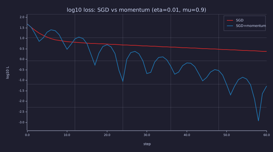
The blue curve is not monotone: it ripples with a period of about 7 steps. The run is deterministic, so this is not noise — it is the second-order pole, worked out just below.
Plain SGD ends at loss \(2.3950\) — the flat direction has barely moved — while momentum reaches \(0.0533\), about 45× lower. The velocity buffer turns the small, consistent \(\theta_2\) gradient into a step roughly \(1/(1-\mu) = 10\times\) larger, so the flat direction finally makes progress; meanwhile the sign-flipping steep-direction gradient averages toward zero. This is the same demo as sgd_vs_momentum.rlab. Now read the ripple off the characteristic polynomial printed above. For \(a = 20\), \(\eta = 0.01\), \(\mu = 0.9\) the poles are 0.850 ± 0.421j: magnitude \(\sqrt{\mu} = 0.949\) (a 5 % decay per step) at an angle of \(26.4\) degrees, i.e. one full oscillation of \(\theta_1\) every \(13.7\) steps. The loss is quadratic in \(\theta_1\), so it rings at twice the frequency — a period of \(6.8\) steps, which is what the figure shows. The Systems lens below places these poles on the unit circle for three curvatures.
Adam: Per-Parameter Adaptive Learning Rates
Theory
Adam keeps two EMAs:
- The first moment \(\mathbf{m}_t = \beta_1 \mathbf{m}_{t-1} + (1 - \beta_1)\mathbf{g}_t\) — like momentum, but normalised to a true mean.
- The second moment \(\mathbf{v}_t = \beta_2 \mathbf{v}_{t-1} + (1 - \beta_2)\mathbf{g}_t^2\) — an EMA of squared gradients (per coordinate).
A parameter whose gradient has been large recently will have a large \(v_t\) in that slot; dividing by \(\sqrt{v_t}\) shrinks its effective step. Parameters that rarely receive a strong signal get a bigger step. The update is
\[\hat{\mathbf{m}}_t = \mathbf{m}_t / (1 - \beta_1^t), \qquad \hat{\mathbf{v}}_t = \mathbf{v}_t / (1 - \beta_2^t), \qquad \theta_t = \theta_{t-1} - \eta\,\frac{\hat{\mathbf{m}}_t}{\sqrt{\hat{\mathbf{v}}_t} + \varepsilon}.\]
The hats are bias correction: at \(t = 1\), \(\mathbf{m}_1 = (1-\beta_1)\mathbf{g}_1\) is heavily biased toward zero and \(\mathbf{v}_1 = (1-\beta_2)\mathbf{g}_1^2\) even more so; dividing by \(1 - \beta_1^t\) and \(1 - \beta_2^t\) removes the bias exactly at \(t = 1\) (the hats recover \(\mathbf{g}_1\) and \(\mathbf{g}_1^2\)). The first-moment correction fades fast — \(1 - \beta_1^{50} \approx 0.995\) — but the second-moment correction does not: \(1 - \beta_2^{50} \approx 0.049\) is still a \(\sim 20\times\) rescale, and \(1 - \beta_2^{100} \approx 0.095\) a \(\sim 10\times\) one, because \(\beta_2 = 0.999\) has a half-life of about 693 steps. The \(\hat{\mathbf{v}}_t\) correction stays material for hundreds of steps.
Example — Adam step on the same anisotropic bowl
beta1 = 0.9;
beta2 = 0.999;
eps   = 1e-8;
eta_a = 0.09;

theta_adam = [-2.0, 4.0];
m = [0.0, 0.0];
v = [0.0, 0.0];
path_adam = zeros(n_steps + 1, 2);
path_adam(1, 1) = theta_adam(1);
path_adam(1, 2) = theta_adam(2);

for k = 1:n_steps
  g  = grad(theta_adam);
  m  = beta1 * m + (1 - beta1) * g;
  v  = beta2 * v + (1 - beta2) * (g .* g);
  m_hat = m / (1 - beta1 ^ k);
  v_hat = v / (1 - beta2 ^ k);
  theta_adam = theta_adam - eta_a * m_hat ./ (sqrt(v_hat) + eps);
  path_adam(k + 1, 1) = theta_adam(1);
  path_adam(k + 1, 2) = theta_adam(2);
end

print("Adam final loss:", loss(theta_adam));
print("Adam final theta:", theta_adam);Adam final loss: 0.01694228895693814
Adam final theta: [1×2] 0.005759 0.165078Adam's per-coordinate rescaling lets both directions advance at similar speeds. It drives \(\theta_2\) down to \(0.165\) and \(\theta_1\) to \(0.006\), so the final loss is \(1.6942e-02\) — roughly two orders of magnitude below SGD's \(2.7035\) on the identical 60-step budget. Dividing each coordinate's step by \(\sqrt{\hat{v}_t}\) is what breaks the condition-number bottleneck that traps SGD: the flat coordinate, whose gradient is small but consistent, gets a full-sized step instead of a \(0.9\%\) nudge.
Coupled vs Decoupled Weight Decay
Theory
L2 regularisation and weight decay are two names for the same operation — but only under plain SGD. L2 regularisation adds a penalty \(\tfrac{\lambda}{2}\|\theta\|^2\) to the loss; its gradient contributes \(\lambda\theta\), so vanilla SGD becomes
\[\theta_t = \theta_{t-1} - \eta(\mathbf{g}_t + \lambda\theta_{t-1}) = (1 - \eta\lambda)\,\theta_{t-1} - \eta\,\mathbf{g}_t.\]
The refactored right-hand side shows the equivalence: adding \(\lambda\theta\) to the gradient is multiplying \(\theta\) by \((1 - \eta\lambda)\) each step — a leak toward zero with pole \(1 - \eta\lambda\).
Under Adam the two part ways. Fold \(\lambda\theta\) into the gradient — call this Adam-with-L2 — and it flows through both moment estimates. A large-magnitude parameter picks up a large \(\lambda\theta\) in its \(\mathbf{v}_t\), so its whole update is divided by a correspondingly larger \(\sqrt{\hat{v}_t}\): the decay it feels is rescaled per coordinate by the same \(1/\sqrt{\hat{v}_t}\) that scales the gradient. Loshchilov & Hutter (2017) argued this coupling is the bug — a regulariser ought to shrink every coordinate by the same fraction, not one modulated by each coordinate's gradient history. Their fix decouples the decay, applying it straight to the parameter, outside the moment machinery:
\[\boxed{\text{AdamW: } \theta_t = \theta_{t-1} - \eta\left(\frac{\hat{\mathbf{m}}_t}{\sqrt{\hat{\mathbf{v}}_t} + \varepsilon} + \lambda\theta_{t-1}\right).}\]
So AdamW is not "L2 regularisation done right under Adam." It is a genuinely different update from Adam-with-L2 — a leak toward zero applied outside the preconditioner, with the same fractional shrinkage \(\eta\lambda\) for every coordinate, whatever its curvature. The two agree only in the plain-SGD limit. Every published GPT (and most modern transformers) uses AdamW.
Example — Adam vs AdamW with weight decay
A 2D problem whose data loss is minimised at \((1, 5)\), with weight decay pulling back toward the origin. The high-curvature coordinate \(\theta_1\) and the low-curvature \(\theta_2\) experience different effective decays under the coupled vs decoupled implementations, so the two settle at different points.
function g = grad_wd_demo(theta)
  % Loss = 0.5*(theta(1) - 1.0)^2 + 0.5*0.1*(theta(2) - 5.0)^2
  g = [theta(1) - 1.0, 0.1 * (theta(2) - 5.0)];
end
% coupled = 1: Adam-with-L2 — lambda*theta is added to the gradient, so it passes
%              through both moment estimates and the 1/sqrt(v_hat) preconditioner.
% coupled = 0: AdamW — lambda*theta is subtracted outside the moment machinery.
function theta = adam_wd(theta, lambda, coupled, eta, n)
  b1 = 0.9;  b2 = 0.999;  e = 1e-8;
  m = [0.0, 0.0];  v = [0.0, 0.0];
  for k = 1:n
    g = grad_wd_demo(theta) + coupled * lambda * theta;
    m = b1 * m + (1 - b1) * g;
    v = b2 * v + (1 - b2) * (g .* g);
    theta = theta - eta * ((m / (1 - b1 ^ k)) ./ (sqrt(v / (1 - b2 ^ k)) + e) + (1 - coupled) * lambda * theta);
  end
end

lambda_wd = 0.1;  eta_b = 0.1;  n_b = 200;
theta_c = adam_wd([3.0, 3.0], lambda_wd, 1, eta_b, n_b);
theta_d = adam_wd([3.0, 3.0], lambda_wd, 0, eta_b, n_b);
print("Coupled (Adam+L2) final theta:", theta_c);
print("Decoupled (AdamW) final theta:", theta_d);Coupled (Adam+L2) final theta: [1×2] 0.909107 2.499989
Decoupled (AdamW) final theta: [1×2] 0.967226 4.740061The two variants land at different points. The coupled run converges to \((0.909, 2.500)\) — essentially the textbook L2 optimum \(\arg\min\!\big(L + \tfrac{\lambda}{2}\|\theta\|^2\big) = (10/11,\ 5/2) \approx (0.909, 2.500)\). Measured against the data optimum \((1, 5)\), that is a \(9\%\) shrink on the high-curvature \(\theta_1\) but a full \(50\%\) shrink on the low-curvature \(\theta_2\): coupled L2 pulls the low-curvature coordinate far harder, because there the data gradient is too weak to resist the penalty. AdamW instead lands at \((0.967, 4.740)\) — a near-uniform \(3\%\) / \(5\%\) shrink across the two coordinates. That curvature-independent per-step fractional decay is exactly what decoupling buys; it is a different endpoint from coupled L2, not the same one reached more accurately.
Three Trajectories on One Surface
Theory
Plot SGD, Adam, and AdamW paths over the same anisotropic bowl, with the loss level sets drawn in so the ravine is visible. SGD zigzags across the steep axis while crawling along the flat one; Adam glides down the ravine floor; AdamW glides the same way but its weight-decay term adds a constant pull toward the origin, so it settles even closer to it. (The bowl's minimum is itself the origin here, so that pull costs no extra loss.)
Example — Optimiser-trajectory overlay
% AdamW path on the original elongated bowl, with weight decay pulling the
% optimum toward the origin.
lambda_aw = 0.05;
theta_aw = [-2.0, 4.0];
m_aw = [0.0, 0.0];
v_aw = [0.0, 0.0];
path_adamw = zeros(n_steps + 1, 2);
path_adamw(1, 1) = theta_aw(1);
path_adamw(1, 2) = theta_aw(2);
for k = 1:n_steps
  g = grad(theta_aw);
  m_aw = beta1 * m_aw + (1 - beta1) * g;
  v_aw = beta2 * v_aw + (1 - beta2) * (g .* g);
  m_hat = m_aw / (1 - beta1 ^ k);
  v_hat = v_aw / (1 - beta2 ^ k);
  theta_aw = theta_aw - eta_a * (m_hat ./ (sqrt(v_hat) + eps) + lambda_aw * theta_aw);
  path_adamw(k + 1, 1) = theta_aw(1);
  path_adamw(k + 1, 2) = theta_aw(2);
end
print("final ||theta||   Adam:", norm(theta_adam), "   AdamW:", norm(theta_aw));

% Level sets of L = 1/2 (200 x^2 + y^2) under the three paths.  The level c is
% x = ±sqrt((2c - y^2) / 200), drawn with plot() and clipped to the window.
function bowl_levels(a, levels, y_lo, y_hi)
  for c = levels
    yv = linspace(max(-sqrt(2 * c), y_lo), min(sqrt(2 * c), y_hi), 80);
    xv = sqrt((2 * c - yv .^ 2) / a);
    plot(xv, yv, "color", "gray")
    plot(-xv, yv, "color", "gray")
  end
end
lev = [0.5, 2, 5, 10, 20, 40, 80, 160, 400];
figure();
plot(path_sgd(:, 1),   path_sgd(:, 2),   "color", "red",   "label", "SGD")
hold("on")
plot(path_adam(:, 1),  path_adam(:, 2),  "color", "blue",  "label", "Adam")
plot(path_adamw(:, 1), path_adamw(:, 2), "color", "green", "label", "AdamW (λ=0.05)")
bowl_levels(200.0, lev, -1.0, 4.5)
hold("off")
title("Optimiser trajectories on  L = ½(200 θ₁² + θ₂²)")
xlabel("θ₁  (steep direction)")
ylabel("θ₂  (flat direction)")
legend("SGD", "Adam", "AdamW")final ||theta|| Adam: 0.1651787934911096 AdamW: 0.023991551004220756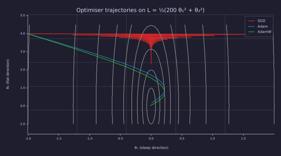
The grey level sets are the ravine: 200× steeper across than along. SGD's red saw blade spans the ravine width; the blue and green paths run down its floor.
SGD's path looks like a saw blade: with \(\eta = 0.009\) the steep coordinate \(\theta_1\) flips sign every step (pole \(1 - \eta \cdot 200 = -0.8\)), so it zigzags while \(\theta_2\) barely drifts. Adam and AdamW both glide smoothly down the floor of the ravine. AdamW ends closer to the origin (\(\|\theta\| = 0.024\)) than Adam (\(\|\theta\| = 0.165\)) because of the constant pull from weight decay — and since the origin is also the loss minimum here, that extra shrinkage costs nothing.
Example — Animated descent
The same three paths, drawn in every third step, make the difference in speed visible: Adam and AdamW reach the ravine floor within a few steps and then slide along it, while SGD is still sawing across the ravine at step 60.
figure();
for k = 4:3:(n_steps + 1)                  % 20 frames, every third step
  plot(path_sgd(1:k, 1),   path_sgd(1:k, 2),   "color", "red",   "label", "SGD")
  hold("on")
  plot(path_adam(1:k, 1),  path_adam(1:k, 2),  "color", "blue",  "label", "Adam")
  plot(path_adamw(1:k, 1), path_adamw(1:k, 2), "color", "green", "label", "AdamW")
  bowl_levels(200.0, lev, -1.0, 4.5)
  hold("off")
  title(sprintf("SGD / Adam / AdamW after %d steps", k - 1))
  frame()
end
saveanim("optimizers.gif", 6)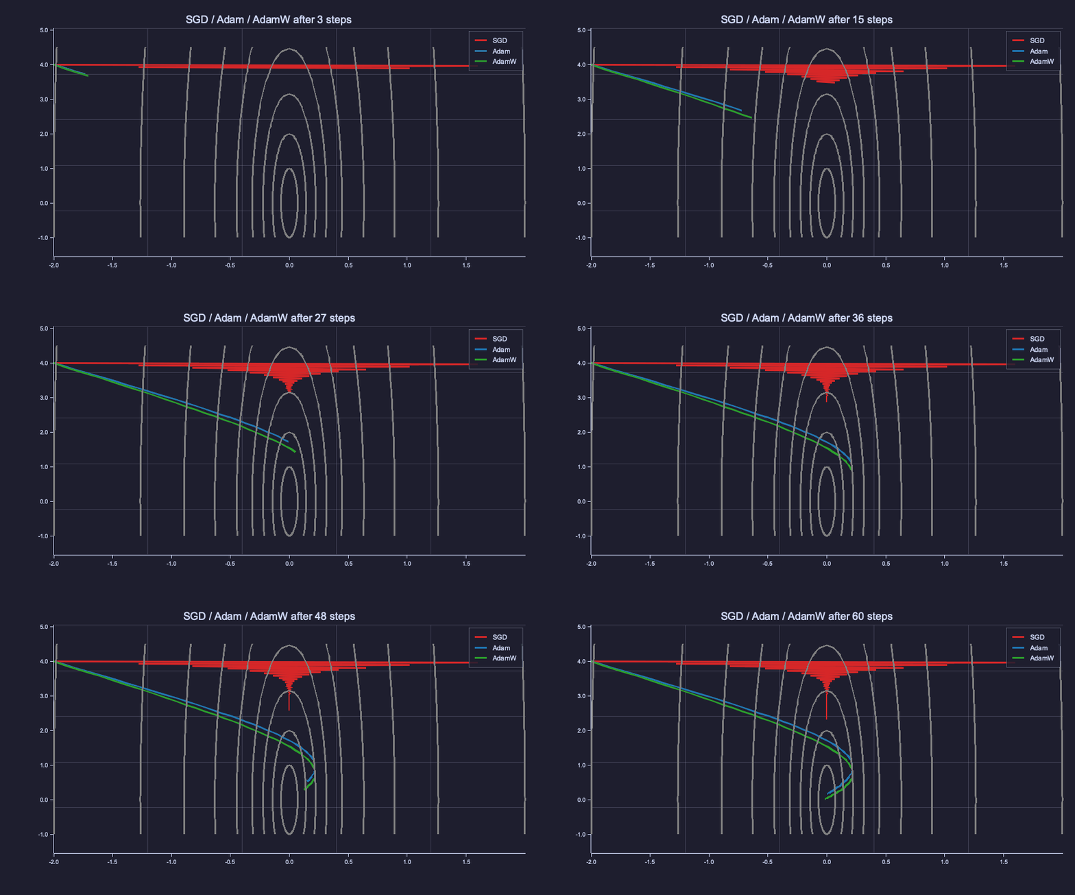
Watch the blue and green paths drop onto the ravine floor (\(\theta_1 \approx 0\)) within about 25 steps and then slide along it toward the origin (\(\theta_2 = 0.17\) at step 60), while the red path is still sawing across the ravine with \(\theta_2 = 2.3\).
Choosing the Hyperparameters
Theory
Three numbers dominate the optimiser's behaviour and they have surprisingly stable defaults across LLM training:
- \(\beta_1 = 0.9\). Half-life \(\log(1/2)/\log(\beta_1) \approx 6.6\) steps. Captures short-term momentum without going stale.
- \(\beta_2 = 0.999\) is the generic Adam default (half-life \(\approx 693\) steps). It tracks per-parameter scale over a long horizon — a parameter's typical gradient magnitude is roughly stationary across many minibatches even when individual gradients are noisy. Large-scale LLM training usually lowers it to \(\beta_2 = 0.95\) (GPT-3, OPT, LLaMA, nanoGPT): at very large batch sizes the long-memory \(0.999\) can destabilise, and \(0.95\) (half-life \(\approx 14\) steps) reacts faster to shifts in gradient scale.
- \(\varepsilon = 10^{-8}\). Prevents division by zero on parameters that have never received a non-trivial gradient (e.g. unused embedding rows for rare tokens).
The learning rate \(\eta\) is the only hyperparameter that requires per-task tuning — and even that is constrained by the warmup-and-decay schedule covered in 17-learning-rate-scheduling. Weight decay \(\lambda\) is typically \(0.1\) for transformer language models (small but non-zero — it does real regularisation work on the embedding and projection matrices).
Engineering Lenses
Signals
Exact. Adam's first moment \(\mathbf{m}_t = \beta_1 \mathbf{m}_{t-1} + (1 - \beta_1)\mathbf{g}_t\) is a one-pole IIR low-pass filter applied to the gradient sequence — one filter per coordinate, the sample index is the training step, the input is in gradient units. Its transfer function is
\[H(z) = \frac{1 - \beta}{1 - \beta z^{-1}},\]
with a single pole at \(z = \beta\), DC gain \(H(1) = 1\), impulse response \((1-\beta)\beta^k\), time constant \(-1/\ln\beta \approx 1/(1-\beta)\) steps and \(-3\) dB corner at \(\omega \approx 1 - \beta\) rad/step, i.e. \((1-\beta)/2\pi\) cycles per step. Heavy-ball momentum \(\mathbf{u}_t = \mu\mathbf{u}_{t-1} + \mathbf{g}_t\) is the same filter without the \((1-\mu)\) normalisation, so its DC gain is \(1/(1-\mu)\). Bias correction is the filter's step response: a constant gradient \(\mathbf{g}\) drives \(\mathbf{m}_t\) to \((1 - \beta^t)\mathbf{g}\), and dividing by \(1 - \beta^t\) removes exactly that deficit.
betas = [0.9, 0.99, 0.999];
n_h = 10000;  n_f = 2048;                          % impulse-response taps, frequency points
ks = 0:(n_h - 1);  t_st = 1:1000;
H_db = zeros(3, n_f - 1);  f3 = zeros(3);
for i = 1:3
  b = betas(i);
  R = freqz((1 - b) * b .^ ks, n_f, 1.0);          % row 1: f in cycles/step; row 2: H(f)
  f  = R(1, 2:n_f);
  Hm = abs(R(2, 2:n_f));
  H_db(i, :) = 20 * log10(Hm);
  f3(i) = f(sum(Hm > 1 / sqrt(2)) + 1);            % first frequency below -3 dB
  print(sprintf("beta = %.3f: DC gain %.4f, -3 dB at %.1e cycles/step (predicted %.1e), tau = %g steps", b, abs(R(2, 1)), f3(i), (1 - b) / (2 * pi), 1 / (1 - b)));
end
R_hb = freqz(0.9 .^ ks, 64, 1.0);
print("heavy ball u = 0.9 u + g: DC gain", abs(R_hb(2, 1)), " = 1/(1 - mu)");

figure();
subplot(1, 2, 1)
semilogx(f, H_db(1, :), "color", "blue",  "label", "beta = 0.9")
hold("on")
semilogx(f, H_db(2, :), "color", "green", "label", "beta = 0.99")
semilogx(f, H_db(3, :), "color", "red",   "label", "beta = 0.999")
hline(-3, "gray", "-3 dB")
hold("off")
title("|H(f)| of the EMA (pole at beta)")
xlabel("cycles per step")
ylabel("dB")
legend("beta = 0.9", "beta = 0.99", "beta = 0.999", "-3 dB")
subplot(1, 2, 2)
plot(t_st, 1 - 0.9 .^ t_st,   "color", "blue",  "label", "beta = 0.9")
hold("on")
plot(t_st, 1 - 0.99 .^ t_st,  "color", "green", "label", "beta = 0.99")
plot(t_st, 1 - 0.999 .^ t_st, "color", "red",   "label", "beta = 0.999")
hold("off")
title("step response 1 - beta^t (bias-correction deficit)")
xlabel("step t")
ylabel("m_t / g")
legend("beta = 0.9", "beta = 0.99", "beta = 0.999")beta = 0.900: DC gain 1.0000, -3 dB at 1.7e-02 cycles/step (predicted 1.6e-02), tau = 10 steps
beta = 0.990: DC gain 1.0000, -3 dB at 1.6e-03 cycles/step (predicted 1.6e-03), tau = 100 steps
beta = 0.999: DC gain 1.0000, -3 dB at 1.8e-04 cycles/step (predicted 1.6e-04), tau = 1000 steps
heavy ball u = 0.9 u + g: DC gain 10.000000000000004 = 1/(1 - mu)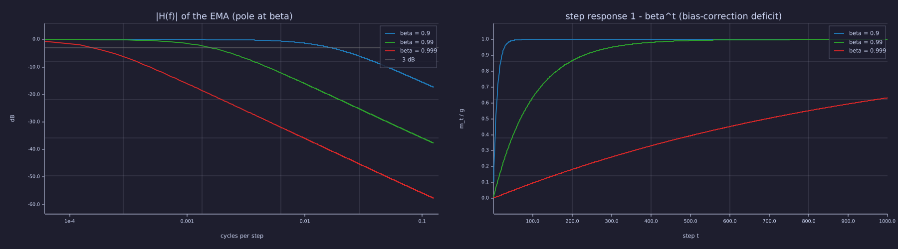
Left: each factor of 10 in \(1-\beta\) slides the corner one decade to the left; all three curves share the same \(-20\) dB/decade slope and unit DC gain. Right: the step response of \(\beta_2 = 0.999\) is still at \(0.095\) after 100 steps — that deficit is the \(\sim 10\times\) bias correction.
The measured corners sit at \(0.0168\), \(0.00165\) and \(0.000183\) cycles per step for \(\beta = 0.9, 0.99, 0.999\) — the predicted \((1-\beta)/2\pi\) to the resolution of the frequency grid. In words: \(\beta_1 = 0.9\) passes gradient components that persist for more than about ten steps and attenuates anything faster, which is exactly the "cancel the sign-flipping steep axis, keep the consistent flat axis" behaviour of the momentum demo.
Systems
Exact. Per coordinate the heavy-ball state is \((\theta_{t-1}, \theta_{t-2})\) and the update law is the second-order recursion derived above, so the poles are the roots of \(z^2 - (1 + \mu - \eta a)z + \mu\). They are real (overdamped) for \(\eta a < (1-\sqrt{\mu})^2\), critically damped at equality, a complex pair at \(\lvert z \rvert = \sqrt{\mu}\) for \((1-\sqrt{\mu})^2 < \eta a < (1+\sqrt{\mu})^2\), and unstable once a real root leaves through \(z = -1\) at \(\eta a = 2(1+\mu)\). Plain SGD's pole for the same mode is the single real number \(1 - \eta a\).
mu_hb = 0.9;  eta_hb = 0.01;
curv = [1, 20, 200];
cols = {"blue", "green", "red"};
th_c = linspace(0, 2 * pi, 361);
figure();
plot(cos(th_c), sin(th_c), "color", "gray", "label", "unit circle")
hold("on")
for i = 1:3
  a_i = curv(i);
  z = roots([1, -(1 + mu_hb - eta_hb * a_i), mu_hb]);
  scatter(real(z), imag(z), "color", cols(i), "label", sprintf("heavy ball, a = %d", a_i))
  print(sprintf("a = %3d: heavy-ball |z| = %.4f at %5.1f deg (period %5.1f steps);  SGD pole 1 - eta a = %+.2f", a_i, abs(z(1)), abs(angle(z(1))) * 180 / pi, 2 * pi / abs(angle(z(1))), 1 - eta_hb * a_i));
end
scatter(1 - eta_hb * curv, [0, 0, 0], "color", "orange", "label", "SGD poles")
hold("off")
title("Heavy-ball poles (mu = 0.9, eta = 0.01) vs SGD poles")
xlabel("Re z")
ylabel("Im z")
legend("unit circle", "a = 1", "a = 20", "a = 200", "SGD")
a_crit = (1 - sqrt(mu_hb)) ^ 2 / eta_hb;
a_max  = 2 * (1 + mu_hb) / eta_hb;
print("critical damping at eta a = (1 - sqrt(mu))^2 =", (1 - sqrt(mu_hb)) ^ 2, " -> a =", a_crit);
print("instability at     eta a = 2 (1 + mu)       =", 2 * (1 + mu_hb), " -> a =", a_max);
g1 = grad([-2.0, 4.0]);                                   % Adam's first step is sign(g): unit size per coordinate
step1 = ((1 - beta1) * g1 / (1 - beta1)) ./ sqrt((1 - beta2) * (g1 .* g1) / (1 - beta2));
print("g_1 =", g1, " ->  m_hat_1 ./ sqrt(v_hat_1) =", step1, " (100:1 input ratio, 1:1 output)");
print("AdamW leak pole 1 - eta lambda at (0.1, 0.1):", 1 - eta_b * lambda_wd, " time constant 1/(eta lambda) =", 1 / (eta_b * lambda_wd), "steps");a = 1: heavy-ball |z| = 0.9487 at 5.1 deg (period 71.3 steps); SGD pole 1 - eta a = +0.99
a = 20: heavy-ball |z| = 0.9487 at 26.4 deg (period 13.7 steps); SGD pole 1 - eta a = +0.80
a = 200: heavy-ball |z| = 0.9487 at 93.0 deg (period 3.9 steps); SGD pole 1 - eta a = -1.00
critical damping at eta a = (1 - sqrt(mu))^2 = 0.002633403898972404 -> a = 0.2633403898972404
instability at eta a = 2 (1 + mu) = 3.8 -> a = 380
g_1 = [1×2] -400.000000 4.000000 -> m_hat_1 ./ sqrt(v_hat_1) = [1×2] -1.000000 1.000000 (100:1 input ratio, 1:1 output)
AdamW leak pole 1 - eta lambda at (0.1, 0.1): 0.99 time constant 1/(eta lambda) = 99.99999999999999 steps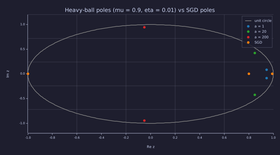
All three heavy-ball pairs lie on the same circle of radius \(\sqrt{\mu} = 0.949\) — the decay rate is curvature-independent from \(a = 0.26\) up to \(a = 380\). Only the angle changes: \(5°\) (a slow 71-step swing), \(26°\) (the 14-step ripple of the momentum demo), \(93°\) (a 4-step ring). SGD's poles spread from \(0.99\) (a 100-step time constant) to \(-1\) (marginal).
Exact. As normalisation: Adam's \(1/\sqrt{\hat{\mathbf{v}}_t}\) is a diagonal preconditioner that divides each coordinate's update by its own recent RMS gradient: a per-coordinate automatic gain control, or equivalently the normalised-LMS step, whose output level is unit regardless of the input level. At \(t = 1\) this is visible in closed form (printed above): \(\hat{\mathbf{m}}_1/\sqrt{\hat{\mathbf{v}}_1} = \mathbf{g}_1/\lvert\mathbf{g}_1\rvert = \operatorname{sign}(\mathbf{g}_1)\), so every coordinate moves by exactly \(\eta\) whatever its gradient. Model. The common gloss "\(1/\sqrt{\hat{\mathbf{v}}}\) approximates the inverse Hessian" is a simplification: \(\sqrt{\hat v}\) has the units of a gradient, not a curvature — it is the square root of the diagonal empirical Fisher (Information lens below). Exact. Decoupled weight decay is a leak: \(\theta \leftarrow (1 - \eta\lambda)\theta\) has pole \(1 - \eta\lambda\) and time constant \(1/(\eta\lambda)\), and "decoupled" means the leak sits outside the preconditioner, so its pole is the same for every coordinate (printed above for the weight-decay demo: \(0.99\), a 100-step time constant).
Information
Exact. With a likelihood loss the gradient is the score \(\partial(-\log p)/\partial\theta\) — for cross-entropy it is \(\mathbf{p} - \mathbf{y}\) (15-backpropagation); for the Gaussian likelihood behind a quadratic loss (03-cross-entropy-loss) it is \(\nabla L\) plus the sensor noise. The expected outer product of the score is the Fisher information, and its diagonal is \(\mathbb{E}[g_i^2] = (\mathbb{E}\,g_i)^2 + \operatorname{Var}\,g_i\). Adam's \(\hat{\mathbf{v}}\) is an EMA estimate of exactly that diagonal — the empirical Fisher, evaluated at the current \(\theta\) over the gradients actually seen — so \(1/\sqrt{\hat v_i}\) divides each coordinate by its RMS score. Near a noisy minimum the mean term vanishes and \(\hat v_i \to \operatorname{Var}\,g_i\): the divisor is pure noise power, and \(\hat m_i/\sqrt{\hat v_i}\) is a signal-to-noise ratio. Model. "\(1/\sqrt{\hat{\mathbf{v}}} \approx\) inverse Hessian" fails on the numbers below: the two coordinates' \(\sqrt{\hat v}\) differ by a factor of about 3, not the Hessian's 200. Run Adam on the \(a = 200\) bowl with \(\sigma = 0.5\) gradient noise (the setting of optimizer_comparison.rlab), using the LLM value \(\beta_2 = 0.95\) so that \(\hat{\mathbf{v}}\) has a 20-step memory and actually tracks the gradient statistics:
seed(16);
sigma = 0.5;  beta2_llm = 0.95;  n_i = 600;
th_i = [-2.0, 4.0];  m_i = [0.0, 0.0];  v_i = [0.0, 0.0];
G = zeros(n_i, 2);  S = zeros(n_i, 2);
for k = 1:n_i
  g = grad(th_i) + sigma * randn(2);              % score sample = true gradient + sensor noise
  m_i = beta1 * m_i + (1 - beta1) * g;
  v_i = beta2_llm * v_i + (1 - beta2_llm) * (g .* g);
  m_hat = m_i / (1 - beta1 ^ k);
  v_hat = v_i / (1 - beta2_llm ^ k);
  G(k, :) = g;
  S(k, :) = m_hat ./ sqrt(v_hat);
  th_i = th_i - eta_a * m_hat ./ (sqrt(v_hat) + eps);
end
w = 401:600;
g1 = reshape(G(w, 1), 1, 200);  g2 = reshape(G(w, 2), 1, 200);
s1 = reshape(S(w, 1), 1, 200);  s2 = reshape(S(w, 2), 1, 200);
var_g = [std(g1) ^ 2, std(g2) ^ 2];
snr_rms = [sqrt(mean(s1 .^ 2)), sqrt(mean(s2 .^ 2))];
print("v_hat at t = 600                 :", v_hat);
print("mean g^2 over steps 401-600      :", [mean(g1 .^ 2), mean(g2 .^ 2)]);
print("  = mean(g)^2 + var(g)           :", [mean(g1) ^ 2, mean(g2) ^ 2], " + ", var_g, "   (sigma^2 =", sigma ^ 2, ")");
print("rms of m_hat ./ sqrt(v_hat)      :", snr_rms, "   white-noise prediction sqrt((1-b1)/(1+b1)) =", sqrt((1 - beta1) / (1 + beta1)));
print("sqrt(v_hat) ratio, coord 1 : 2 :", sqrt(v_hat(1) / v_hat(2)), " Hessian ratio a/b = 200");v_hat at t = 600 : [1×2] 3.321424 0.285148
mean g^2 over steps 401-600 : [1×2] 2.839760 0.279113
= mean(g)^2 + var(g) : [1×2] 0.000091 0.000020 + [1×2] 2.853939 0.280495 (sigma^2 = 0.25 )
rms of m_hat ./ sqrt(v_hat) : [1×2] 0.094679 0.238139 white-noise prediction sqrt((1-b1)/(1+b1)) = 0.22941573387056174
sqrt(v_hat) ratio, coord 1 : 2 : 3.4129295220721456 Hessian ratio a/b = 200The estimate \(\hat{\mathbf{v}}\) and the directly measured second moment agree coordinate by coordinate, and the mean-squared term is negligible against the variance: at the noisy minimum \(\hat{\mathbf{v}}\) is the noise power. For the flat coordinate that power is \(\sigma^2 = 0.25\) — pure sensor noise — and its step ratio has RMS \(0.24\), matching the \(\sqrt{(1-\beta_1)/(1+\beta_1)} = 0.229\) that a one-pole filter of white noise produces: at a noisy minimum Adam keeps moving each coordinate by about \(0.23\,\eta\) per step. That residual is the noise floor the learning-rate decay of 17-learning-rate-scheduling exists to remove. The steep coordinate's variance, \(2.85\), is far above \(\sigma^2\): Adam's own \(\eta\)-sized jitter across the ravine (\(\theta_1\) oscillating by \(\sim 10^{-2}\), times \(a = 200\)) generates most of that coordinate's "noise" — the optimiser's limit cycle, which 18-training-loop meets again in the gradient-norm diagnostic.
Key Takeaways
- Vanilla SGD on a mode with curvature \(a\) has pole \(1 - \eta a\): stable iff \(\eta < 2/a\), so the steepest direction sets the learning rate and the flattest direction crawls.
- Momentum is a one-pole low-pass filter on the gradient (pole \(\beta\), time constant \(1/(1-\beta)\)); heavy ball turns each mode into a second-order system whose complex poles all sit at \(\lvert z \rvert = \sqrt{\mu}\) — curvature-independent decay, at the price of ringing.
- Adam maintains a first-moment EMA \(\mathbf{m}_t\) (momentum) and a second-moment EMA \(\mathbf{v}_t\) (per-parameter RMS gradient — a diagonal empirical Fisher), with bias correction that divides out the filter's step-response deficit \(1 - \beta^t\); the \(\beta_2\) correction stays material for hundreds of steps.
- AdamW applies weight decay as a leak outside the preconditioner: \(\lambda\theta\) is subtracted directly from the parameter, not folded into \(\mathbf{v}_t\), so every coordinate shrinks by the same fraction \(\eta\lambda\) per step. It is a different update from Adam-with-L2, not a more accurate one.
- The hyperparameters \(\beta_1 = 0.9\), \(\varepsilon = 10^{-8}\), \(\lambda = 0.1\) are stable defaults across transformer training. \(\beta_2 = 0.999\) is the generic Adam default, but published large-scale LLM training (GPT-3, OPT, LLaMA, nanoGPT) uses \(\beta_2 = 0.95\) for stability at large batch sizes.
Standalone Scripts
| Script | What it computes |
|---|---|
sgd_vs_momentum.rlab | SGD vs heavy-ball momentum on the \(a = 20\) bowl (noiseless, 60 steps — the notebook's numbers); loss curves and trajectories |
adam_step.rlab | one Adam step in detail with bias correction; shows the \(\hat{\mathbf{m}}\) factor reaching \(\approx 1\) within a few steps while the \(\hat{\mathbf{v}}\) factor lags (\(\beta_2\) half-life \(\approx 693\) steps) |
optimizer_comparison.rlab | SGD vs Adam vs AdamW trajectories on loss contours. It differs from the notebook overlay: it adds \(\sigma = 0.5\) gradient noise and runs 80 steps, so its final losses (Adam \(\approx 0.071\), AdamW \(\approx 0.035\)) are not the noiseless numbers above |
momentum_filter.rlab | the EMA as a one-pole filter: freqz magnitude in dB and step response for \(\beta \in \{0.9, 0.99, 0.999\}\); measured \(-3\) dB corners and time constants |
heavy_ball_poles.rlab | heavy-ball poles via roots for \(a \in \{1, 20, 200\}\) on the unit circle beside the SGD poles; critical-damping and instability curvatures |
adam_snr.rlab | noisy Adam run with \(\beta_2 = 0.95\): \(\hat{\mathbf{v}}\) vs the measured gradient second moment, per-coordinate step ratio (SNR), and \(\sqrt{\hat v}\) vs the Hessian |
Run all with make lesson-16 (or rustlab run lessons/16-adamw-optimizer/<name>.rlab).
Expected Numerical Outputs Summary
| Variable | Expected Value |
|---|---|
loss(theta_sgd) after 60 SGD steps (\(a = 200\), \(\eta = 0.009\)) | 2.7035 (\(\theta_2\) stuck at 2.325; \(\theta_1\) converged) |
loss_s(end), loss_v(end) (\(a = 20\), \(\eta = 0.01\), \(\mu = 0.9\)) | 2.3950 vs 0.0533 — momentum ≈ 45× lower |
| heavy-ball poles for \(a = 20\) | \(0.850 \pm 0.421j\): \(\lvert z \rvert = \sqrt{0.9} = 0.9487\), angle 26.4°, period 13.7 steps in \(\theta_1\), 6.8 in the loss |
loss(theta_adam) after 60 Adam steps | 0.0169 (~160× below SGD) |
theta_c, theta_d (coupled vs decoupled decay) | (0.909, 2.500) vs (0.967, 4.740) |
norm(theta_adam), norm(theta_aw) (overlay) | 0.165 vs 0.024 |
| bias correction \(1 - \beta_1\) at \(t = 1\); \(1 - \beta_2^{100}\) | 0.1; 0.095 (still a 10× rescale — not negligible) |
| EMA \(-3\) dB corners, \(\beta = 0.9 / 0.99 / 0.999\) | 1.7e-2 / 1.6e-3 / 1.8e-4 cycles per step (\(\approx (1-\beta)/2\pi\)); DC gain 1.000; heavy-ball DC gain 10 |
| critical-damping / instability curvature at \(\eta = 0.01\), \(\mu = 0.9\) | $a = $ 0.263 / 380 |
snr_rms(2), sqrt(v_hat(1)/v_hat(2)) (noisy run, \(\beta_2 = 0.95\)) | ≈ 0.24 (white-noise value 0.229); ≈ 3.4 (Hessian ratio 200) |
Exercises
- Why bias correction matters. At \(t = 1\), write \(\mathbf{m}_1\) and \(\mathbf{v}_1\) in terms of \(\mathbf{g}_1\) and confirm \(\hat{\mathbf{m}}_1 = \mathbf{g}_1\), \(\hat{\mathbf{v}}_1 = \mathbf{g}_1^2\). Now suppose you skipped both corrections: show that the raw first step \(\mathbf{m}_1 / \sqrt{\mathbf{v}_1}\) exceeds the corrected step \(\hat{\mathbf{m}}_1 / \sqrt{\hat{\mathbf{v}}_1}\) by a factor \((1 - \beta_1)/\sqrt{1 - \beta_2}\). Evaluate it at \((\beta_1, \beta_2) = (0.9, 0.999)\) — is the uncorrected first step too large or too small, and by how much?
- Tuning \(\beta_2\). Re-run
adam_step.rlabwith \(\beta_2 = 0.9\). Does the optimiser still converge as quickly? In filter terms, what happened to the second moment's time constant, and why does a long horizon matter for a scale estimate but not for a direction estimate? - Why \(\varepsilon\) inside the square root vs outside. The original Adam paper uses \(\hat{\mathbf{m}} / (\sqrt{\hat{\mathbf{v}}} + \varepsilon)\). What changes if you write \(\hat{\mathbf{m}} / \sqrt{\hat{\mathbf{v}} + \varepsilon}\)? On parameters with \(\hat{v} \to 0\), which version gives a saner step size?
- Critical damping by hand. For \(\mu = 0.9\) and \(a = 20\), find the \(\eta\) at which the heavy-ball poles become real (\(\eta a = (1-\sqrt\mu)^2\)) and the \(\eta\) at which one of them reaches \(-1\). Re-run the momentum demo at both values and describe the loss curves.
- Loss surface intuition.
optimizer_comparison.rlabalready runs at condition number 200. Push it further to \(L = 0.5(1000\theta_1^2 + \theta_2^2)\): what is the new SGD stability bound \(2/a\), and what learning rate must SGD use? Does Adam's \(\eta\) need to change at all? Re-run and compare the final losses.
What's next
17-learning-rate-scheduling covers the learning-rate schedule that wraps every step of the optimiser. Real LLM training uses a short linear warmup followed by a long cosine decay. In the language of this lesson that is gain scheduling: a time-varying \(\eta_t\) moves every pole derived here along the real axis and around the unit circle during the run — and the residual \(0.23\,\eta\) jitter measured under the Information lens is why the gain must come down at the end.