Lesson 08: Scaled Dot-Product Attention
07-context-and-naive-averaging rewrote causal prefix averaging as a matrix multiply \(\bar{\mathbf{X}} = \mathbf{W}\mathbf{X}\) where \(\mathbf{W}\) was lower-triangular with fixed \(1/t\) weights — a causal FIR filter along the token axis. Attention keeps the same skeleton but makes the taps learned and data-dependent. This lesson derives the full operation:
\[\mathrm{Attn}(\mathbf{Q},\mathbf{K},\mathbf{V}) \;=\; \mathrm{softmax}\!\left(\frac{\mathbf{Q}\mathbf{K}^\top}{\sqrt{d_k}} + \mathbf{M}\right)\mathbf{V}.\]
One renaming, stated once: Lesson 07's mixing matrix \(\mathbf{W}\) is called \(\mathbf{A}\) from here on (rows = query time \(t\), columns = key time \(i \le t\)), and \(\mathbf{W}\) now denotes a learned projection such as \(\mathbf{W}_Q\).
Learning Objectives
- Define the query, key, and value matrices \(\mathbf{Q}, \mathbf{K}, \mathbf{V}\) derived from a sequence of embeddings via three learned linear projections, and say why they are three different projections.
- Write and explain the scaled dot-product attention equation \(\mathrm{Attn}(\mathbf{Q},\mathbf{K},\mathbf{V}) = \mathrm{softmax}\!\left(\tfrac{\mathbf{Q}\mathbf{K}^\top}{\sqrt{d_k}}\right)\mathbf{V}\) one piece at a time.
- Motivate the \(1/\sqrt{d_k}\) scale from the variance of a dot product of independent vectors, and measure what it does to the entropy of an attention row.
- Apply a causal mask so position \(t\) cannot see tokens at positions \(> t\) and verify the resulting attention matrix is lower-triangular.
- Read attention as a correlation receiver, a kernel smoother and an associative memory, and read a hand-built attention matrix entry by entry.
Background
Embeddings as dense row vectors and the dot product as a correlator from 04-embeddings-and-similarity. Softmax, entropy and probability row-normalisation from 02-probability-and-softmax and 03-cross-entropy-loss. Linear layers from 06-linear-layers-and-gradient-descent, where a layer was written \(\mathbf{y} = \mathbf{x}\mathbf{W} + \mathbf{b}\) with \(\mathbf{x}\) a row vector. Here rows are tokens, and the same right-multiplication applies to every row of \(\mathbf{X}\) at once: \(\mathbf{X}\mathbf{W}\) applies one linear map to the whole sequence. Causal prefix averaging as a time-varying FIR filter from 07-context-and-naive-averaging. Entropies are computed with lib/info.rlab.
Queries, Keys, Values
Theory
Given an input \(\mathbf{X} \in \mathbb{R}^{T \times d_{\text{model}}}\) (row \(t\) is the embedding of token \(t\)), three learned linear projections produce three matrices:
\[\mathbf{Q} = \mathbf{X}\mathbf{W}_Q \in \mathbb{R}^{T \times d_k}, \quad \mathbf{K} = \mathbf{X}\mathbf{W}_K \in \mathbb{R}^{T \times d_k}, \quad \mathbf{V} = \mathbf{X}\mathbf{W}_V \in \mathbb{R}^{T \times d_v}.\]
- \(\mathbf{W}_Q, \mathbf{W}_K \in \mathbb{R}^{d_{\text{model}} \times d_k}\) — project each embedding into a query and key vector.
- \(\mathbf{W}_V \in \mathbb{R}^{d_{\text{model}} \times d_v}\) — project into a value vector.
Each token emits three vectors: a query (what it's looking for), a key (what it advertises), a value (what it contributes if selected). They are separate projections because what a token asks for, what it advertises, and what it hands over are three different things — a pronoun asks for a noun, advertises "pronoun", and hands over whatever features the next layer needs. The parameters are learned by gradient descent (06-linear-layers-and-gradient-descent); once trained, they encode which features matter for prediction.
Example — Hand-crafted Q and K with an interpretable pattern
T = 5;
d_k = 4;
scale = 1.0 / sqrt(d_k);

% Hand-crafted Q, K designed so the attention pattern is interpretable.
% Key 1 advertises feature 1 loudly; queries 2 and 4 look for feature 1;
% query 3 looks for feature 2, which key 2 advertises; query 5 wants a bit of both.
K = [ 2.0, 0.0, 0.0, 0.0;
      0.0, 2.0, 0.0, 0.0;
      0.0, 0.0, 2.0, 0.0;
      1.0, 1.0, 0.0, 0.0;
      0.0, 0.0, 1.0, 1.0 ];

Q = [ 1.0, 0.0, 0.0, 0.0;
      1.0, 0.0, 0.0, 0.0;
      0.0, 1.0, 0.0, 0.0;
      1.0, 0.0, 0.0, 0.0;
      0.5, 0.5, 0.0, 0.0 ];
The pay-off of this design is read off \(\mathbf{A}\) below, entry by entry.
The Score Matrix
Theory
Entry \((t, i)\) of \(\mathbf{S} = \mathbf{Q}\mathbf{K}^\top\) is the dot product \(\mathbf{q}_t \cdot \mathbf{k}_i\) — a raw similarity between query \(t\) and key \(i\).
Why divide by \(\sqrt{d_k}\)? If \(\mathbf{q}\) and \(\mathbf{k}\) are independent of each other and each has \(d_k\) i.i.d. components with mean 0 and variance 1, then \(\mathbf{q}\cdot\mathbf{k} = \sum_{j=1}^{d_k} q_j k_j\) has variance \(d_k\) (sum of \(d_k\) independent unit-variance products) and so standard deviation \(\sqrt{d_k}\). As \(d_k\) grows, raw dot products grow too, softmax becomes razor-sharp (one entry approaches 1, others approach 0), and gradients vanish. Scaling by \(1/\sqrt{d_k}\) keeps the input to softmax at roughly unit variance regardless of dimension:
\[\mathbf{S}_{\text{scaled}} = \frac{\mathbf{Q}\mathbf{K}^\top}{\sqrt{d_k}}.\]
Example — Compute the scaled score matrix
S = Q * K' * scale;Example — Empirical variance grows with \(d_k\), and softmax saturates without scaling
The variance argument above is the central justification for the \(1/\sqrt{d_k}\) factor in the original Attention Is All You Need paper. Verify it numerically: sample i.i.d. \(\mathcal{N}(0, 1)\) vectors at three dimensions and measure \(\mathrm{Var}(\mathbf{q}\cdot\mathbf{k})\). (Names ending in _v are local to this example so the global T, Q, K from earlier blocks stay intact for the sections below.)
seed(8);
n_samples = 5000;
dks = [4, 64, 512];
for kk = 1:3
  dk_v = dks(kk);
  dots_v = zeros(n_samples);
  for s = 1:n_samples
    q_v = randn(1, dk_v);
    k_v = randn(1, dk_v);
    dots_v(s) = sum(q_v .* k_v);
  end
  var_v = mean(dots_v .^ 2);          % variance, since dots have mean ~0
  ratio_v = var_v / dk_v;             % variance of (q.k)/sqrt(d_k) is ratio_v
  print("d_k =", dk_v, "  Var(q.k) =", var_v, "  Var(q.k) / d_k =", ratio_v);
endd_k = 4 Var(q.k) = 3.9421480253630032 Var(q.k) / d_k = 0.9855370063407508
d_k = 64 Var(q.k) = 64.25729915186785 Var(q.k) / d_k = 1.0040202992479352
d_k = 512 Var(q.k) = 528.3374583922757 Var(q.k) / d_k = 1.0319090984224135The expected ratio is \(\approx 1\) at every \(d_k\) — the variance scales linearly with \(d_k\), which is why dividing by \(\sqrt{d_k}\) restores unit-variance scores regardless of dimension. The downstream consequence, measured on one row at \(d_k = 512\) with the row's entropy in bits as the yardstick:
seed(8);
dk_v = 512;
T_v  = 8;
Q_v = randn(T_v, dk_v);
K_v = randn(T_v, dk_v);
S_unscaled_v = Q_v * K_v';                            % raw dot products, variance ~512
S_scaled_v   = Q_v * K_v' * (1.0 / sqrt(dk_v));        % unit variance after scaling
A_unscaled_v = softmax(S_unscaled_v(1, :));            % row 1 of the attention distribution
A_scaled_v   = softmax(S_scaled_v(1, :));
H_unscaled_v = entropy_bits(A_unscaled_v);
H_scaled_v   = entropy_bits(A_scaled_v);
print("unscaled: max A =", max(A_unscaled_v), "  H(A) =", H_unscaled_v, "bits");
print("scaled: max A =", max(A_scaled_v), " H(A) =", H_scaled_v, "bits (uniform over 8 =", log2(T_v), "bits)");unscaled: max A = 0.9999999999999583 H(A) = 0.000000000001914218322257698 bits
scaled: max A = 0.5235101584047486 H(A) = 2.1887527342740865 bits (uniform over 8 = 3 bits)Unscaled, the row puts \(\approx 1.0\) on one position and carries \(1.9e-12\) bits — a hard selector. Scaled, the same row spreads (max \(0.52\), \(2.19\) of the \(3\) available bits) and the model can actually blend values across positions. Preview of 15-backpropagation: the diagonal of the softmax Jacobian is \(p(1-p)\), which goes to 0 as \(p \to 1\), so a saturated row passes no gradient through any column, the argmax included — training stalls. The \(\sqrt{d_k}\) factor is what keeps attention trainable in practice. The Information lens below animates the whole transition from flat to one-hot.
The Causal Mask
Theory
For a language model, token \(t\) must not see tokens at positions \(i > t\). Add a mask \(\mathbf{M}\) with entries \(-\infty\) above the diagonal and 0 elsewhere:
\[M_{t, i} = \begin{cases} 0 & i \le t \\ -\infty & i > t. \end{cases}\]
In code the mask is a large finite negative number (\(-10^9\)) rather than literal \(-\infty\). For a causal mask that is a convenience, not a necessity: every row keeps its diagonal, so the row maximum that a numerically stable softmax subtracts is finite, \(-\infty - \max\) is still \(-\infty\), and \(\exp(-\infty) = 0\) exactly. The genuine failure case is a row that is masked entirely — padding positions in batched training — where \(-\infty - (-\infty) = \text{NaN}\). The other honest reason is portability: frameworks add the mask in the tensor's own dtype, and a finite "very negative" constant chosen per dtype (\(-10^9\) would itself overflow fp16) works for float and integer masks alike.
Example — Apply the mask to S
NEG_INF = -1.0e9;
M = NEG_INF * (1 - cumsum(eye(T), 1));   % 0 on / below the diagonal, -1e9 above (Lesson 07's mask trick)
S_masked = S + M;
Row-wise Softmax → Attention Weights
Theory
Applying softmax to each row turns the scores into a probability distribution. The \(-10^9\) entries become exactly 0:
\[A_{t, i} = \frac{\exp(\tilde S_{t, i})}{\sum_{j=1}^{T} \exp(\tilde S_{t, j})}.\]
Example — Build A and read it back
% softmax(M) acts on each row independently (dim = 2 default, ML convention),
% so the whole attention matrix is one call; the per-row max subtraction is automatic.
A = softmax(S_masked);
print("A =");
print(A);A =
Matrix(5x5)
[1.000000, 0.000000, 0.000000, 0.000000, 0.000000]
[0.731059, 0.268941, 0.000000, 0.000000, 0.000000]
[0.211942, 0.576117, 0.211942, 0.000000, 0.000000]
[0.426933, 0.157060, 0.157060, 0.258948, 0.000000]
[0.237357, 0.237357, 0.143964, 0.237357, 0.143964]row_sums = zeros(T);
for t = 1:T
row_sums(t) = sum(A(t, :));
end
A_1_1 = A(1, 1);
max_upper = 0.0;
for i = 1:T
for j = (i + 1):T
if A(i, j) > max_upper
max_upper = A(i, j);
end
end
end
print("A(1,1) =", A_1_1, " row sums =", row_sums);
print("largest upper-triangle entry =", max_upper);A(1,1) = 1 row sums = [1×5] 1.000000 1.000000 1.000000 1.000000 1.000000
largest upper-triangle entry = 0Now read the design back. Row 2 puts \(0.73\) on \(t_1\) (query 2 asked for feature 1; key 1 has it) against \(0.5\) under uniform averaging. Row 3 puts \(0.58\) on \(t_2\), the key advertising feature 2. Row 4 puts \(0.43\) on \(t_1\) — a token three positions back, retrieved by content, against the \(0.25\) that Lesson 07's \(1/4\) would give; its own half-strength key earns it \(0.26\). Row 5's half-and-half query ties \(t_1\), \(t_2\) and \(t_4\) at \(0.24\) each. Token 1 can only attend to itself, so \(A_{1,1} = 1.0000\); every row sums to 1; the largest entry in the upper triangle is \(0.00e+00\) — zero, as causality requires.
Example — Three-stage pipeline heatmap
Both axes are token positions: rows are the query positions \(t\) (which token is asking) and columns are the key positions \(i\) (which token is being read).
positions = {"t1", "t2", "t3", "t4", "t5"};
M_ind = (M < 0);   % 1 where the causal mask blocks attention, 0 elsewhere

figure();
subplot(1, 3, 1)
heatmap(positions, positions, S, "Scaled scores S = Q K^T / sqrt(d_k)", "viridis")
subplot(1, 3, 2)
heatmap(positions, positions, M_ind, "Causal mask (1 = blocked)", "viridis")
subplot(1, 3, 3)
heatmap(positions, positions, A, "Attention weights A = softmax_row(S + M)", "viridis")
Left: a score lights up wherever a query's feature meets a key's feature (column \(t_4\) is warm everywhere because key 4 carries both features). Middle: the blocked upper triangle. Right: the same triangle as Lesson 07's \(\mathbf{W}\), but with mass pulled onto \(t_1\) in rows 2 and 4 and onto \(t_2\) in row 3.
Full Pipeline: X → Q, K, V → Output
Theory
Wire it all together: three projections, the score → mask → softmax chain, and the value mix \(\mathbf{O} = \mathbf{A}\mathbf{V}\). Shapes on every edge:
Only the \(T \times T\) boxes mix along the token axis; every other box is a per-token linear map. That is why the causal mask lives in exactly one place.
Example — Project X into Q, K, V
Five tokens, read as "mat was soft, it was …". The columns of \(\mathbf{X}\) are hand-labelled features [noun, verb, adjective, pronoun, spare, spare], one-hot so the arithmetic can be followed by eye. The projections are chosen so that a pronoun asks for a noun but advertises "pronoun" — which is exactly why queries and keys must be different maps.
d_model = 6;
d_v = 4;
tokens = {"t1 mat", "t2 was", "t3 soft", "t4 it", "t5 was"};
X = [ 1, 0, 0, 0, 0, 0;     % mat   (noun)
      0, 1, 0, 0, 0, 0;     % was   (verb)
      0, 0, 1, 0, 0, 0;     % soft  (adjective)
      0, 0, 0, 1, 0, 0;     % it    (pronoun)
      0, 1, 0, 0, 0, 0 ];   % was   (verb, again)

% W_Q: what each kind of token LOOKS FOR. Query dim 1 = "a noun", dim 2 = "a pronoun".
W_Q = zeros(d_model, d_k);
W_Q(2, :) = [2, 2, 0, 0];   % a verb looks for its subject: a noun or a pronoun
W_Q(3, :) = [2, 0, 0, 0];   % an adjective looks for the noun it describes
W_Q(4, :) = [2, 0, 0, 0];   % a pronoun looks for the noun it stands for

% W_K: what each kind of token ADVERTISES, on the same dims.
W_K = zeros(d_model, d_k);
W_K(1, :) = [3, 0, 0, 0];   % a noun advertises "noun"
W_K(4, :) = [0, 3, 0, 0];   % a pronoun advertises "pronoun"
W_K(2, :) = [0, 0, 3, 0];   % verbs and adjectives advertise on dims no query asks for
W_K(3, :) = [0, 0, 0, 3];

% W_V: what a token HANDS OVER when selected — here its first four features, unchanged.
W_V = [eye(4); zeros(2, 4)];

Q2 = X * W_Q;
K2 = X * W_K;
V2 = X * W_V;
Example — Compute attention weights and output, and read them back
S2 = Q2 * K2' * scale;
M2 = NEG_INF * (1 - cumsum(eye(T), 1));
A2 = softmax(S2 + M2);            % row-wise softmax in one call
O  = A2 * V2;
print("A2 =");
print(A2);
print("O =");
print(O);A2 =
Matrix(5x5)
[1.000000, 0.000000, 0.000000, 0.000000, 0.000000]
[0.952574, 0.047426, 0.000000, 0.000000, 0.000000]
[0.909443, 0.045279, 0.045279, 0.000000, 0.000000]
[0.870049, 0.043317, 0.043317, 0.043317, 0.000000]
[0.465255, 0.023164, 0.023164, 0.465255, 0.023164]
O =
Matrix(5x4)
[1.000000, 0.000000, 0.000000, 0.000000]
[0.952574, 0.047426, 0.000000, 0.000000]
[0.909443, 0.045279, 0.045279, 0.000000]
[0.870049, 0.043317, 0.043317, 0.043317]
[0.465255, 0.046327, 0.023164, 0.465255]diff_row1 = max(abs(O(1, :) - V2(1, :)));
n_params_qkv = 3 * d_model * d_k;
print("max |O(1, :) - V(1, :)| =", diff_row1, " params 3 * d_model * d_k =", n_params_qkv);max |O(1, :) - V(1, :)| = 0 params 3 * d_model * d_k = 72Query 4 (it) meets key 1 (mat) with score \(2 \cdot 3 / \sqrt{4} = 3\) and every other visible key with score 0, so \(A_{4,1} = e^{3}/(e^{3} + 3) = 0.870\): token 4 retrieves token 1, three positions back, against the \(0.25\) uniform averaging would give. That is content-based retrieval — the thing Lesson 07 could not do. Row 2's verb finds its subject (\(0.95\) on mat), row 3's adjective does too (\(0.91\)), and row 5's second verb has two candidate subjects and splits \(0.465\) / \(0.465\) between mat and it — attention represents the ambiguity instead of guessing. In the output, row 4 is \(0.87\) of mat's value plus three slivers of \(0.043\): the it row now carries the noun's content. Row 1 of \(\mathbf{O}\) equals row 1 of \(\mathbf{V}\) (token 1 attends only to itself): \(\max|\mathbf{O}_1 - \mathbf{V}_1| = 0.00e+00\). The block's learnable parameters are \(3 \cdot d_{\text{model}} \cdot d_k = 3 \cdot 6 \cdot 4 = 72\) — a count that does not depend on the sequence length \(T\).
Example — Attention weights and output heatmaps
out_dims = {"noun", "verb", "adj", "pron"};

figure();
subplot(1, 2, 1)
heatmap(tokens, tokens, A2, "Attention weights A (rows: query token, cols: key token)", "viridis")
subplot(1, 2, 2)
heatmap(out_dims, tokens, O, "Output O = A V  (rows: tokens, cols: value features)", "viridis")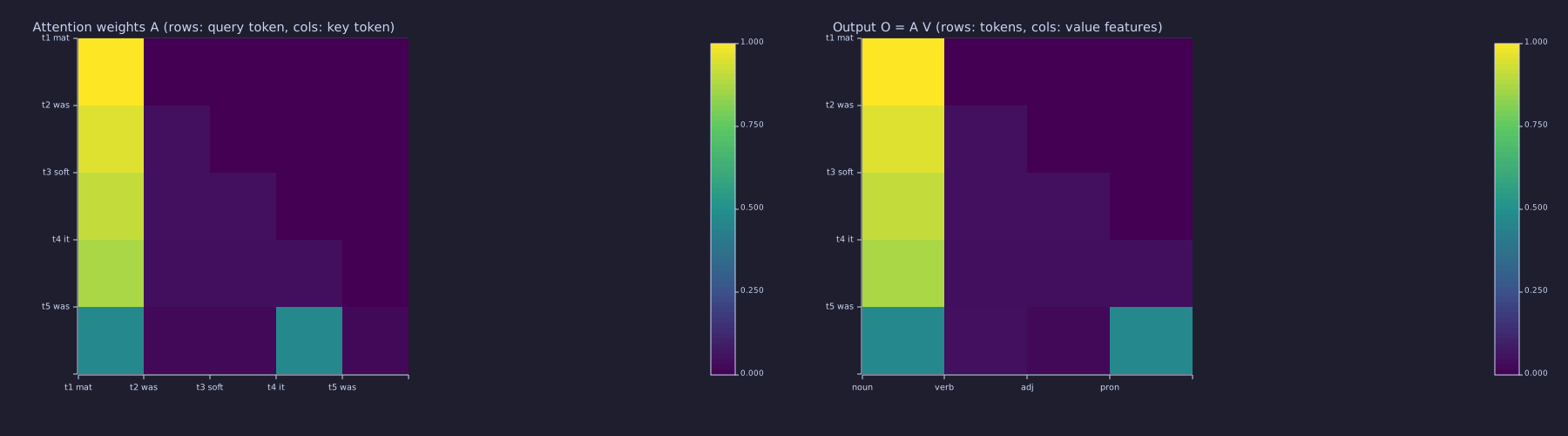
The bright cell at (t4 it, t1 mat) is the retrieval; compare with the flat rows of Lesson 07's \(\mathbf{W}\). Row t5 was has two bright cells — the unresolved subject. On the right, the noun column is lit for every token that looked one up.
Engineering Lenses
Attention has no state of its own inside a single forward call — the stored keys and values only become a state when generation reuses them as the KV cache (21-sampling-and-generation) — so no systems reading is given here; the training-time dynamics of these weights are 15-backpropagation and 16-adamw-optimizer.
Signals
Exact. Correlation receiver. \(s_{t,i} = \mathbf{q}_t \cdot \mathbf{k}_i\) correlates one template (the query) against every stored waveform (the keys) — the matched-filter operation of 04-embeddings-and-similarity, applied \(t\) times per row. Softmax is a soft-argmax detector on the correlator outputs, and \(1/\sqrt{d_k}\) normalises the noise floor: for independent unit-variance components the correlator output has variance \(d_k\) (measured above), so the scale returns it to unit variance whatever the dimension.
Exact. Kernel smoother. Row \(t\) of the output is a Nadaraya–Watson estimate,
\[\mathbf{o}_t = \frac{\sum_{i \le t} \kappa(\mathbf{q}_t, \mathbf{k}_i)\, \mathbf{v}_i}{\sum_{i \le t} \kappa(\mathbf{q}_t, \mathbf{k}_i)}, \qquad \kappa(\mathbf{q}, \mathbf{k}) = \exp\!\big(\mathbf{q}\cdot\mathbf{k} / \sqrt{d_k}\big),\]
and softmax's normalisation is the smoother's denominator. Lesson 07 is the special case \(\kappa \equiv 1\) — a box kernel: set \(\mathbf{W}_Q = \mathbf{W}_K = \mathbf{0}\) and \(\mathbf{A}\) collapses to \(\mathbf{W}_{\text{avg}}\) exactly. Two lessons, one formula.
% Nadaraya-Watson form of row 4, computed from the raw kernel weights
t = 4;
num = zeros(1, d_v);
den = 0.0;
for i = 1:t
  kappa = exp(S2(t, i));                  % S2 already carries the 1/sqrt(d_k)
  num = num + kappa * V2(i, :);
  den = den + kappa;
end
diff_nw = max(abs(num / den - O(t, :)));
print("max|Nadaraya-Watson row 4 - O(4, :)| =", diff_nw);

% Box kernel: zero projections give Lesson 07's averaging matrix back
A_box = softmax(zeros(T, T) + M2);
W_avg = cumsum(eye(T), 1) ./ repmat((1:T)', 1, T);
diff_box = max(reshape(abs(A_box - W_avg), 1, T * T));
print("max|A(W_Q = W_K = 0) - W_avg| =", diff_box);max|Nadaraya-Watson row 4 - O(4, :)| = 0.00000000000000033306690738754696
max|A(W_Q = W_K = 0) - W_avg| = 0Model. Associative memory. Keys are addresses, values are contents, the query is a probe, and the read-out is a convex combination of contents weighted by address match. Row 4 above is one lookup: probe "a noun" → address mat → content \(\mathbf{v}_1\), with \(0.87\) fidelity; row 5 is a probe that matches two addresses.
Analogy. Because the taps of the FIR filter are computed from the signal itself, attention behaves like an adaptive filter — but there is no error-driven tap update at inference time; the adaptation is instantaneous and feed-forward.
Information
Exact. The row entropy \(H(\mathbf{A}_t) = -\sum_i A_{t,i}\log_2 A_{t,i}\) (bits) measures how spread row \(t\) is, and \(2^{H}\) is the effective number of tokens attended. Lesson 07's uniform row has \(H = \log_2 t\), the maximum; a hard lookup has \(H = 0\). Computed for both matrices of this lesson:
H_A  = row_entropies_bits(A);
H_A2 = row_entropies_bits(A2);
print(" t  log2(t) |  hand-crafted A: H(A_t)  2^H  |  pipeline A2: H(A_t)  2^H");
for t = 1:T
  fprintf(" %d   %.2f   |        %.2f            %.2f  |        %.2f          %.2f\n", t, log2(t), H_A(t), 2 ^ H_A(t), H_A2(t), 2 ^ H_A2(t));
endt log2(t) | hand-crafted A: H(A_t) 2^H | pipeline A2: H(A_t) 2^H
1 0.00 | 0.00 1.00 | 0.00 1.00
2 1.00 | 0.84 1.79 | 0.28 1.21
3 1.58 | 1.41 2.65 | 0.53 1.44
4 2.00 | 1.87 3.65 | 0.76 1.70
5 2.32 | 2.28 4.87 | 1.40 2.65Row 4 of the hand-crafted \(\mathbf{A}\) attends to \(3.65\) effective tokens of the 4 available; the pipeline's row 4 attends to \(1.70\) — the lookup is nearly hard. Row 5 of \(\mathbf{A}_2\) sits at \(2.65\): the two candidate subjects plus a little leakage. Trained heads typically sit far below \(\log_2 t\); these entropies are the measurement that says how far.
Exact. \(\mathbf{S} = \mathbf{Q}\mathbf{K}^\top\) is a bilinear form, so \(\operatorname{rank}\mathbf{S} \le \min(\operatorname{rank}\mathbf{Q}, \operatorname{rank}\mathbf{K}) \le d_k\) however long the sequence:
print("rank(S)  =", rank(S),  "  rank(Q)  =", rank(Q),  "  rank(K)  =", rank(K),  "  d_k =", d_k);
print("rank(S2) =", rank(S2), " rank(Q2) =", rank(Q2), " rank(K2) =", rank(K2));rank(S) = 2 rank(Q) = 2 rank(K) = 4 d_k = 4
rank(S2) = 2 rank(Q2) = 2 rank(K2) = 4Both score matrices have rank 2: the queries only ever ask two questions. A head with \(d_k\) dimensions can pose at most \(d_k\) independent questions, which is why 09-multi-head-attention can afford \(d_k = 2\) per head and why a single head cannot realise an arbitrary \(T \times T\) pattern. (Mask and softmax act after \(\mathbf{S}\), so \(\mathbf{A}\) itself is generally full rank; the budget is on the scores.)
Exact. The scale is an entropy knob. One query row against 8 random keys, scores at unit variance, softmaxed at multiples \(c\) of the \(1/\sqrt{d_k}\) operating point:
seed(16);
T_g = 8;
dk_g = 16;
q_g = randn(1, dk_g);
K_g = randn(T_g, dk_g);
s_g = q_g * K_g' / sqrt(dk_g);              % one query row against 8 keys, unit-variance scores
keys_g = {"t1", "t2", "t3", "t4", "t5", "t6", "t7", "t8"};
scales = linspace(0.1, 3.0, 30);
figure();
for k = 1:length(scales)
  c = scales(k);
  a = softmax(c * s_g);
  subplot(1, 2, 1)
  bar(keys_g, c * s_g)
  ylim([-3, 6])
  title(sprintf("scores  c * q.k / sqrt(d_k),   c = %.2f", c))
  subplot(1, 2, 2)
  bar(keys_g, a)
  ylim([0, 1])
  title(sprintf("softmax row:  H(A_t) = %.2f bits  (uniform = 3.00)", entropy_bits(a)))
  frame();
end
saveanim("softmax_sharpening.gif", 6)
H_c01 = entropy_bits(softmax(0.1 * s_g));
H_c1  = entropy_bits(softmax(s_g));
H_c3  = entropy_bits(softmax(3.0 * s_g));
print("H(A_t) at c = 0.1, 1, 3:", H_c01, H_c1, H_c3, "bits (log2 8 =", log2(T_g), ")");H(A_t) at c = 0.1, 1, 3: 2.995300634107477 2.2559471769069237 0.1687290966557756 bits (log2 8 = 3 )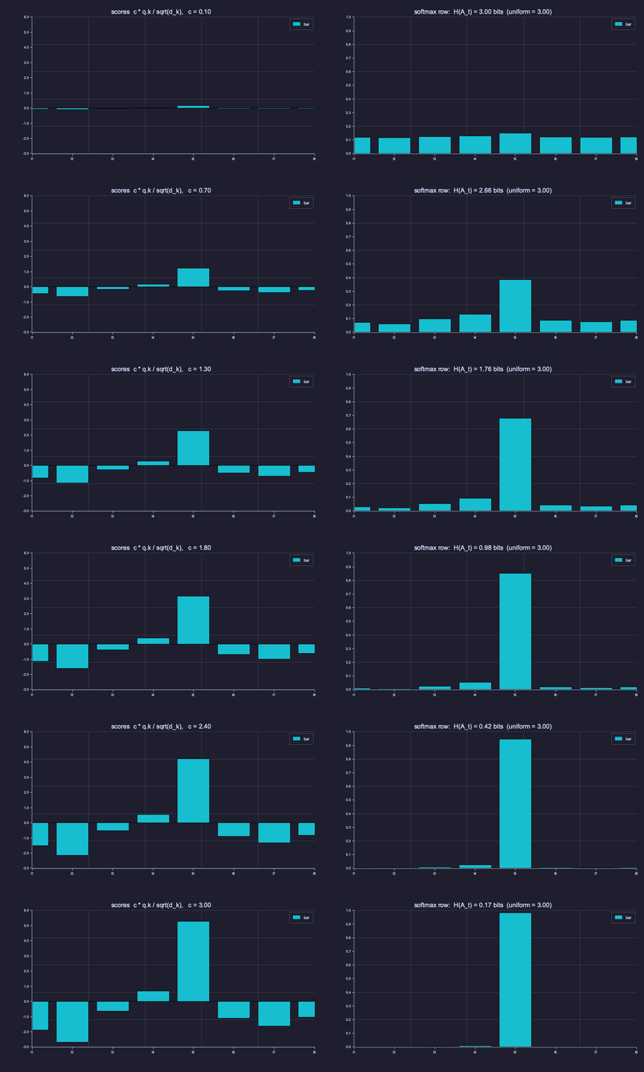
At \(c = 0.1\) the row is flat (\(3.00\) bits — all 8 tokens); at \(c = 1\), the \(1/\sqrt{d_k}\) operating point, it is \(2.26\) bits; by \(c = 3\) it is nearly one-hot on \(t_5\) (\(0.17\) bits). The scores' ordering never changes — only how many bits the row keeps.
Model. The floor \(H(X_{t+1} \mid X_{1..t})\) from 05-bigram-language-model and 07-context-and-naive-averaging is what any predictor must approach. Uniform averaging collapses the prefix into one bag and dilutes most of \(I(X_{t+1};\, X_{1..t})\); per-row re-weighting lets \(\mathbf{o}_t\) stay informative about \(X_{t+1}\) for whichever prior token carries the information — the \(0.5\) bits the toy corpus lost to the bigram are recoverable by a head that puts its mass on the first token. The row entropies above are the per-position measurement of how selective that routing is.
Key Takeaways
- Queries, keys, values are three linear projections of the same input \(\mathbf{X}\) — self-attention means they all come from the same sequence — and they differ because asking, advertising and handing over are different jobs.
- The score matrix \(\mathbf{S} = \mathbf{Q}\mathbf{K}^\top / \sqrt{d_k}\) is a bank of correlator outputs of rank \(\le d_k\); the \(1/\sqrt{d_k}\) scale keeps it at unit variance, which is what keeps the row entropy — and the gradient — alive.
- The causal mask zeros out future positions so position \(t\) can only look at tokens \(1..t\); \(-10^9\) stands in for \(-\infty\) for fully-masked rows and dtype portability, not because \(\exp(-\infty)\) misbehaves.
- Softmax is row-wise: each row of \(\mathbf{A}\) is a distribution over the first \(t\) tokens, and \(\mathbf{O} = \mathbf{A}\mathbf{V}\) is a Nadaraya–Watson kernel smoother whose box-kernel special case is Lesson 07's prefix average.
- The parameter count of one self-attention block (\(\mathbf{W}_Q, \mathbf{W}_K, \mathbf{W}_V\)) is \(3 \cdot d_{\text{model}} \cdot d_k\) when \(d_v = d_k\) (in general \(d_{\text{model}}(2 d_k + d_v)\)), independent of sequence length.
Standalone Scripts
| Script | What it computes |
|---|---|
attention_weights.rlab | scores → masked → softmax pipeline on hand-crafted \(\mathbf{Q}, \mathbf{K}\); \(\mathbf{A}\) printed and read back entry by entry; three-stage heatmap |
attention_output.rlab | full \(X \to Q, K, V \to O\) pipeline on the five-token mat was soft it was example; token 4 retrieves token 1; heatmaps |
attention_entropy.rlab | row entropies \(H(\mathbf{A}_t)\) against \(\log_2 t\) and \(2^H\); \(\operatorname{rank}\mathbf{S} \le d_k\); Nadaraya–Watson and box-kernel checks; bar chart of entropies |
softmax_sharpening.rlab | GIF of one query row's scores and softmax as the scale sweeps \(0.1 \to 3\), \(H(\mathbf{A}_t)\) in the title |
Run all with make lesson-08 (or rustlab run lessons/08-scaled-dot-product-attention/<name>.rlab).
Expected Numerical Outputs Summary
| Variable | Expected Value |
|---|---|
scale (= \(1/\sqrt{4}\)) | 0.5 |
Var(q.k) / d_k at \(d_k = 4 / 64 / 512\) | ≈ 0.99 / 1.00 / 1.03 (variance grows linearly with \(d_k\)) |
max A_unscaled, H_unscaled_v at \(d_k = 512\) | ≈ 1.0, ≈ 0 bits (saturated) |
max A_scaled, H_scaled_v at \(d_k = 512\) | ≈ 0.52, ≈ 2.19 bits of 3 (well-spread) |
A(2,1), A(3,2), A(4,1), A(5,1) | 0.731, 0.576, 0.427, 0.237 |
A_1_1; row_sums; max_upper | 1.0000; 1.0 each; ≈ 0 |
A2(4,1) (it → mat); A2(2,1); A2(5,1) = A2(5,4) | 0.870; 0.953; 0.465 |
O(4, :) | [0.870, 0.043, 0.043, 0.043] |
diff_row1 (\(\max\lvert\mathbf{O}_1 - \mathbf{V}_1\rvert\)); n_params_qkv | ≈ 0; 72 |
diff_nw, diff_box | ≈ 0 (machine epsilon), 0 |
H_A (hand-crafted rows 1–5) | 0, 0.84, 1.41, 1.87, 2.28 bits vs \(\log_2 t\) = 0, 1, 1.58, 2, 2.32 |
H_A2 (pipeline rows 1–5) | 0, 0.28, 0.53, 0.76, 1.40 bits |
rank(S), rank(S2); d_k | 2, 2; 4 |
H_c01, H_c1, H_c3 (animation row) | 3.00, 2.26, 0.17 bits |
Exercises
- The scale matters. Remove the \(1/\sqrt{d_k}\) factor in
attention_weights.rlab. How do the row entropies change when \(d_k = 4\)? Try doubling the diagonal of \(\mathbf{Q}\) and \(\mathbf{K}\) to make the dot products larger — what does softmax do to \(H(\mathbf{A}_t)\) as the scores grow? - Drop the mask. Disable the causal mask in
attention_weights.rlab. Confirm that token 1 now attends to future tokens. Why does this break language-model training? - Self vs. cross. In
attention_output.rlab, let the keys and values come from a different sequence \(\mathbf{Y} \in \mathbb{R}^{T' \times d_{\text{model}}}\) (cross-attention) while queries still come from \(\mathbf{X}\). Which shapes change in the pipeline diagram? Does a causal mask still make sense, and when? - Parameter counting. For \(d_{\text{model}} = 384\), \(d_k = d_v = 64\), compute the parameter count of \(\mathbf{W}_Q, \mathbf{W}_K, \mathbf{W}_V\) together. Add an output projection \(\mathbf{W}_O \in \mathbb{R}^{d_v \times d_{\text{model}}}\) — what's the total now?
- Complexity. The score matrix \(\mathbf{S} = \mathbf{Q}\mathbf{K}^\top\) has \(T \times T\) entries. How does the cost of computing \(\mathbf{S}\) scale with sequence length \(T\)? Why is this the bottleneck that motivates efficient attention variants (FlashAttention, sliding window, linear attention)?
What's next
09-multi-head-attention runs multiple attention heads in parallel, each with its own \(\mathbf{W}_Q^{(h)}, \mathbf{W}_K^{(h)}, \mathbf{W}_V^{(h)}\), then concatenates their outputs and projects them back to \(d_{\text{model}}\) — a filter bank of rank-\(d_k\) mixers. Different heads learn to specialise — one might track syntax, another long-range references — without any explicit supervision telling them which is which.