Lesson 13: The Transformer Block
You now have every piece a transformer needs: multi-head attention (Lesson 09), positional encoding (Lesson 10), the feed-forward sublayer (Lesson 11), and LayerNorm + residual connections (Lesson 12). This lesson assembles them into the transformer block — the unit that gets stacked \(N\) times to form a full GPT — and adds the one mental model the pieces do not give you on their own: the block acts on a \(T \times d_{\text{model}}\) signal along two different axes, and only one of its sublayers can move information along time.
Learning Objectives
- Write the Pre-LN transformer block forward pass as a single equation and identify each sublayer.
- Read the block as a signal-flow graph and trace the \((T, d_{\text{model}})\) shape along every edge; confirm input shape equals output shape.
- Name the two mixing axes — attention mixes along time (rows), the FFN along channels (columns) — and demonstrate it with a perturbation test.
- Implement one full block end-to-end, stack blocks, and track the residual stream's magnitude and per-block gain with and without the \(1/\sqrt{2N}\) branch scaling.
- Compute the parameter count per block and identify which sublayer dominates.
Background
Multi-head attention from Lesson 09. FFN with \(d_{\text{ff}} = 4 d_{\text{model}}\) from Lesson 11. LayerNorm and the Pre-LN residual convention from Lesson 12. Causal mask from Lesson 08. Notation follows Lesson 00: tokens are rows (time \(t = 1, \dots, T\)), features are columns (channels), layers act by right-multiplication. No new mathematics — only assembly.
Pre-LN Block: The Forward Pass
Theory
The modern (Pre-LN) transformer block is two sublayers, each wrapped in LayerNorm-then-sublayer-then-residual:
\[\begin{aligned} \mathbf{H}_{\text{mid}} &= \mathbf{H}_{\text{in}} + \mathrm{MHA}\!\left(\mathrm{LN}_1(\mathbf{H}_{\text{in}})\right), \\ \mathbf{H}_{\text{out}} &= \mathbf{H}_{\text{mid}} + \mathrm{FFN}\!\left(\mathrm{LN}_2(\mathbf{H}_{\text{mid}})\right). \end{aligned}\]
As a signal-flow graph, with the tensor shape on every edge:
Follow the bottom path: \(\mathbf{H}_{\text{in}}\) reaches \(\mathbf{H}_{\text{out}}\) untouched through the two + nodes. Each sublayer only adds a correction to that stream — the "residual stream" of Lesson 12, now wired concretely. Every edge on the stream carries a \((T, d_{\text{model}})\) matrix.
The two mixing axes. Think of \(\mathbf{H} \in \mathbb{R}^{T \times d_{\text{model}}}\) as a signal with two axes: down the rows is time (token position \(t\)), across the columns are channels (feature dimensions). The two sublayers move information along different axes:
- Attention mixes rows. Row \(t\) of \(\mathrm{MHA}(\cdot)\) is a weighted sum of other rows \(i \le t\) — the attention matrix \(\mathbf{A}_h \in \mathbb{R}^{T \times T}\) multiplies from the left. It is the only operation in the whole block (indeed the whole GPT) that lets token \(t\) see token \(i \ne t\).
- The FFN mixes columns. It acts on each row independently: \(\mathbf{W}_1\) and \(\mathbf{W}_2\) multiply from the right and recombine the channels of one token. It never reads another row.
LayerNorm also acts per row (it standardises each token's channels), so the only time-axis coupling in the block is \(\mathbf{A}_h\). The perturbation test in the two mixing axes section below makes this visible: bump one entry of token 3 and the attention sublayer's response spreads to rows \(3, 4\) (never \(1, 2\) — causality), while the FFN's response stays inside row 3 and spreads across all eight channels.
Every tensor along the residual stream has shape \((T, d_{\text{model}})\). Inside MHA the projections temporarily produce \((T, d_k)\) per-head matrices, but the concat + output projection \(\mathbf{W}_O\) collapses them back to \((T, d_{\text{model}})\). Inside FFN the hidden layer briefly widens to \((T, d_{\text{ff}})\) before the second linear projection reduces it. The residual stream's width is invariant — that is what makes blocks stackable without intervening reshape logic.
Example — Configure dimensions and initialise weights
Use a small but realistic config for the worked example: \(T = 4\), \(d_{\text{model}} = 8\), \(H = 2\) heads of \(d_k = 4\) each, \(d_{\text{ff}} = 32\).
seed(13);
T = 4;
d_model = 8;
H_heads = 2;
d_k = d_model / H_heads;     % 4
d_ff = 4 * d_model;          % 32

H_in = randn(T, d_model);

% Multi-head attention weights — packed as full d_model × d_model matrices.
% Each head will read a contiguous d_k-wide slice of the columns.
W_Q = randn(d_model, d_model) * (1.0 / sqrt(d_model));
W_K = randn(d_model, d_model) * (1.0 / sqrt(d_model));
W_V = randn(d_model, d_model) * (1.0 / sqrt(d_model));
W_O = randn(d_model, d_model) * (1.0 / sqrt(d_model));

% FFN weights with He init for the GELU pre-activation
W_ff1 = randn(d_model, d_ff) * sqrt(2.0 / d_model);
W_ff2 = randn(d_ff,    d_model) * sqrt(2.0 / d_ff);

print("H_in shape:                      ", size(H_in));
print("W_{Q,K,V,O} shape (each):        ", size(W_Q));
print("W_ff1 shape (d_model -> d_ff):   ", size(W_ff1));
print("W_ff2 shape (d_ff -> d_model): ", size(W_ff2));H_in shape: [1×2] 4.000000 8.000000
W_{Q,K,V,O} shape (each): [1×2] 8.000000 8.000000
W_ff1 shape (d_model -> d_ff): [1×2] 8.000000 32.000000
W_ff2 shape (d_ff -> d_model): [1×2] 32.000000 8.000000LayerNorm in this notebook uses \(\boldsymbol{\gamma} = \mathbf{1}, \boldsymbol{\beta} = \mathbf{0}\) — pure standardisation, no learned affine. Real implementations carry \((\boldsymbol{\gamma}, \boldsymbol{\beta})\) as small parameter vectors; the parameter count below lists them separately and the forward pass skips them for clarity.
Sublayer 1: Pre-LN Multi-Head Self-Attention
Theory
The first sublayer is
\[\mathbf{A} = \mathrm{MHA}\!\left(\mathrm{LN}_1(\mathbf{H}_{\text{in}})\right), \qquad \mathbf{H}_{\text{mid}} = \mathbf{H}_{\text{in}} + \mathbf{A}.\]
Pre-LN means LayerNorm runs before the projections — the inputs to \(\mathbf{W}_Q, \mathbf{W}_K, \mathbf{W}_V\) are already normalised, so the dot-product scores stay in a sensible range from the very first iteration. The \(1/\sqrt{d_k}\) scale (Lesson 08) handles the rest.
The MHA computation is exactly Lesson 09's: per head, score → mask → softmax → weighted sum → concat → \(\mathbf{W}_O\). The novelty here is just plumbing it inside a residual block. The causal mask and, later, the packaged block come from the shared library lib/transformer.rlab.
Example — LN1, then per-head Q/K/V, attention, concat, project
% LN1: layernorm(M) standardises each row — each token — independently.
H_norm1 = layernorm(H_in);

% Project: same equations as Lesson 08, but applied to the LN'd input
Q = H_norm1 * W_Q;       % (T, d_model)
K = H_norm1 * W_K;
V = H_norm1 * W_V;

M_mask = causal_mask(T);          % 0 on/below the diagonal, -1e9 above
scale = 1.0 / sqrt(d_k);
out_concat = zeros(T, d_model);

for h = 1:H_heads
  c_lo = (h - 1) * d_k + 1;     % first column belonging to head h
  c_hi = h * d_k;               % last column belonging to head h
  Q_h = Q(:, c_lo:c_hi);        % slice head h's d_k columns out of Q, K, V
  K_h = K(:, c_lo:c_hi);
  V_h = V(:, c_lo:c_hi);
  S = Q_h * K_h' * scale + M_mask;
  A_h = softmax(S);             % row-wise softmax: one tap vector per query
  O_h = A_h * V_h;
  out_concat(:, c_lo:c_hi) = O_h;   % head h's output goes into its slice of the concat
end

A_out = out_concat * W_O;     % (T, d_model)
print("LN1(H_in) shape:                 ", size(H_norm1));
print("MHA output shape: ", size(A_out));LN1(H_in) shape: [1×2] 4.000000 8.000000
MHA output shape: [1×2] 4.000000 8.000000Both LN1 and the MHA output are \((T, d_{\text{model}}) = (4, 8)\) — same as the input. The per-head \((T, d_k)\) matrices live only inside the loop.
Example — First residual addition
H_mid = H_in + A_out;
print("H_mid shape (after first residual):", size(H_mid));
print("H_mid row 1 (first 4 values): ", H_mid(1, 1), H_mid(1, 2), H_mid(1, 3), H_mid(1, 4));H_mid shape (after first residual): [1×2] 4.000000 8.000000
H_mid row 1 (first 4 values): 1.114650853792557 -1.3444806749068605 1.0992947175874568 0.2117387088439008The residual restores the original \(\mathbf{H}_{\text{in}}\) signal that LN1 had standardised away. Future blocks will read \(\mathbf{H}_{\text{mid}}\) — the unnormalised residual stream — and apply LN to it again from scratch.
Sublayer 2: Pre-LN Feed-Forward
Theory
Same wrapper, different sublayer:
\[\mathbf{F} = \mathrm{FFN}\!\left(\mathrm{LN}_2(\mathbf{H}_{\text{mid}})\right), \qquad \mathbf{H}_{\text{out}} = \mathbf{H}_{\text{mid}} + \mathbf{F}.\]
In the row convention used throughout the course, the FFN is
\[\mathrm{FFN}(\mathbf{X}) = \mathrm{GELU}\!\left(\mathbf{X}\mathbf{W}_1 + \mathbf{1}\mathbf{b}_1^{\top}\right)\mathbf{W}_2 + \mathbf{1}\mathbf{b}_2^{\top}, \qquad \mathbf{W}_1 \in \mathbb{R}^{d_{\text{model}} \times d_{\text{ff}}},\; \mathbf{W}_2 \in \mathbb{R}^{d_{\text{ff}} \times d_{\text{model}}},\]
applied to every row of \(\mathbf{X}\) independently (Lesson 11); \(\mathbf{1}\mathbf{b}^{\top}\) broadcasts a bias row to all \(T\) tokens. Biases are omitted in the code here.
Example — LN2, FFN, second residual
% LayerNorm again — one standardisation per token.
H_norm2 = layernorm(H_mid);

F_pre  = H_norm2 * W_ff1;     % (T, d_ff)
F_post = gelu(F_pre);         % (T, d_ff), still
F_out  = F_post * W_ff2;      % (T, d_model)

H_out = H_mid + F_out;        % residual addition

print("LN2(H_mid) shape:                ", size(H_norm2));
print("FFN hidden  shape (T, d_ff):     ", size(F_pre));
print("FFN output  shape (T, d_model):  ", size(F_out));
print("Block output H_out shape: ", size(H_out));LN2(H_mid) shape: [1×2] 4.000000 8.000000
FFN hidden shape (T, d_ff): [1×2] 4.000000 32.000000
FFN output shape (T, d_model): [1×2] 4.000000 8.000000
Block output H_out shape: [1×2] 4.000000 8.000000The FFN hidden temporarily widens to \((T, d_{\text{ff}}) = (4, 32)\), then contracts back to \((T, d_{\text{model}}) = (4, 8)\). The block's input and output have identical shape, \((4, 8)\). Stacking blocks just means feeding H_out as the next block's H_in.
Example — Magnitude tracking through the block
print("|H_in|  =", norm(H_in));
print("|H_mid| =", norm(H_mid));
print("|H_out| =", norm(H_out));
print("|MHA contribution|  / |H_in|  =", norm(A_out) / norm(H_in));
print("|FFN contribution| / |H_mid| =", norm(F_out) / norm(H_mid));|H_in| = 6.069769106017517
|H_mid| = 9.195808939486904
|H_out| = 10.544696449259169
|MHA contribution| / |H_in| = 0.9873622796827375
|FFN contribution| / |H_mid| = 0.5208642158653086At this lesson's initialisation the sublayer contributions are not small perturbations. The MHA branch is about the same size as the residual stream it feeds into (\(\|\mathrm{MHA}\| / \|\mathbf{H}_{\text{in}}\| \approx 0.99\)); the FFN branch is a bit smaller (\(\approx 0.52\), because its two He-scaled projections contract the variance). Adding a branch of comparable magnitude to the stream grows the norm roughly like the square root of the number of accumulated terms: \(\|\mathbf{H}_{\text{in}}\| = 6.07\) becomes \(\|\mathbf{H}_{\text{mid}}\| = 9.20\) after the first residual and \(\|\mathbf{H}_{\text{out}}\| = 10.54\) after the second. Production GPTs keep these ratios well below 1 on purpose — they shrink each residual-branch output projection at initialisation (nanoGPT divides its variance by \(2N\), i.e. scales the weights by \(1/\sqrt{2N}\); see Lesson 14's initialization sidebar) precisely so a deep stack's residual stream stays bounded. The Systems lens below runs that experiment on an 8-block stack. Training then scales each contribution up where it helps and down where it doesn't.
Example — Visualise the residual stream at each stage
Rather than three nearly identical pictures of the stream, plot the input and the two corrections the block adds to it, on their own signed colour scales.
feat = {"1", "2", "3", "4", "5", "6", "7", "8"};   % channel labels
tok  = {"1", "2", "3", "4"};                       % token (time) labels
figure();
subplot(1, 3, 1)
heatmap(feat, tok, H_in, "H_in", "viridis")
subplot(1, 3, 2)
heatmap(feat, tok, A_out, "MHA correction A_out", "viridis")
subplot(1, 3, 3)
heatmap(feat, tok, F_out, "FFN correction F_out", "viridis")
Rows are tokens \(t = 1..4\), columns channels \(1..8\); colour is the signed value. The MHA correction has a visible column structure (channels 1 and 5 light up for every token — \(\mathbf{W}_O\) writes its output into the same channels regardless of \(t\)), while the FFN correction varies row by row. Neither panel resembles \(\mathbf{H}_{\text{in}}\): the block adds new content instead of rescaling what was there.
The Two Mixing Axes
Theory
The claim in the opening section is precise: \(\mathrm{MHA}\) is the only operation whose row \(t\) depends on rows \(i \ne t\), and — because of the causal mask — only on rows \(i < t\). Write the sublayers as maps on the whole matrix. For any row-wise map \(g\) (LayerNorm, the FFN, a right-multiplication),
\[g(\mathbf{H})_{t,:} = g(\mathbf{H}_{t,:}) \quad \text{(depends on row } t \text{ only)},\]
whereas for a head, \((\mathbf{A}_h \mathbf{V}_h)_{t,:} = \sum_{i \le t} A_h(t, i)\, \mathbf{V}_h(i, :)\) depends on every earlier row. The cleanest test is a perturbation: change one input entry of token 3 and record which output rows move. A row-wise map can only move row 3; a causal time-mixing map can move rows \(3, 4, \dots, T\) and must leave rows \(1, 2\) exactly unchanged.
Example — Perturb token 3 at the input of each sublayer
Two thin wrappers (hidden) evaluate just the MHA sublayer and just the FFN sublayer on an arbitrary input; the test is six lines.
H_p = H_in;
H_p(3, 1) = H_p(3, 1) + 1.0;                   % bump channel 1 of token 3 at the MHA input
dA = attn_sublayer(H_p, W_Q, W_K, W_V, W_O, H_heads, M_mask) - A_out;
H_mid_p = H_mid;
H_mid_p(3, 1) = H_mid_p(3, 1) + 1.0;           % same bump at the FFN input
dF = ffn_sublayer(H_mid_p, W_ff1, W_ff2) - F_out;
print("sum |dA_out| per token (MHA response):", sum(abs(dA), 2)');
print("sum |dF_out| per token (FFN response):", sum(abs(dF), 2)');
print("max |dA_out| on tokens 1-2:", max(max(abs(dA(1:2, :)))), "   channels of token 3 touched by the FFN:", sum(abs(dF(3, :)) > 0), "of", d_model);
figure();
subplot(1, 2, 1)
heatmap(feat, tok, dA, "MHA response to a bump at token 3", "viridis")
subplot(1, 2, 2)
heatmap(feat, tok, dF, "FFN response to a bump at token 3", "viridis")sum |dA_out| per token (MHA response): Matrix(1x4)
[0.000000, 0.000000, 0.775304, 0.351612]
sum |dF_out| per token (FFN response): Matrix(1x4)
[0.000000, 0.000000, 1.758853, 0.000000]
max |dA_out| on tokens 1-2: 0 channels of token 3 touched by the FFN: 8 of 8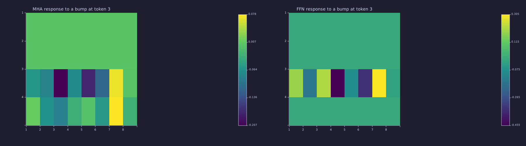
Rows are tokens, columns channels, colour the signed change. Left: the change propagates down the time axis — rows 3 and 4 move, rows 1 and 2 are exactly zero (the causal mask forbids them from seeing token 3). Right: the change stays in row 3 and spreads across all 8 channels — one perturbed channel was recombined into every channel through \(\mathbf{W}_1\), GELU and \(\mathbf{W}_2\). That is the whole division of labour inside a transformer: attention routes along time, the FFN computes along channels.
Stacking Two Blocks
Theory
A real GPT stacks \(N\) identical blocks. "Identical" means same architecture, different parameters per block. Each block has its own \(\mathbf{W}_Q^{(\ell)}, \mathbf{W}_K^{(\ell)}, \mathbf{W}_V^{(\ell)}, \mathbf{W}_O^{(\ell)}, \mathbf{W}_1^{(\ell)}, \mathbf{W}_2^{(\ell)}\) for \(\ell = 1, \dots, N\). The residual stream threads through every block, so block \(\ell\)'s output becomes block \(\ell+1\)'s input — both at width \(d_{\text{model}}\).
Example — Build a second set of weights and run the stack
Block 2 is the same forward pass as the explicit version above, now as a single call to mha_block_forward from the shared library lib/transformer.rlab — the same code, so the numbers match running the loops by hand.
% Block 2 weights — different seed, same architecture
seed(14);
W_Q2 = randn(d_model, d_model) * (1.0 / sqrt(d_model));
W_K2 = randn(d_model, d_model) * (1.0 / sqrt(d_model));
W_V2 = randn(d_model, d_model) * (1.0 / sqrt(d_model));
W_O2 = randn(d_model, d_model) * (1.0 / sqrt(d_model));
W_ff1_2 = randn(d_model, d_ff) * sqrt(2.0 / d_model);
W_ff2_2 = randn(d_ff,    d_model) * sqrt(2.0 / d_ff);

% Run the same block forward pass on H_out as input — one call to the shared
% library function, which is the same code as the explicit version above.
H_out2 = mha_block_forward(H_out, W_Q2, W_K2, W_V2, W_O2, W_ff1_2, W_ff2_2, H_heads, M_mask);

print("After block 1 |H| =", norm(H_out));
print("After block 2 |H| =", norm(H_out2));
print("After block 2 shape:", size(H_out2));After block 1 |H| = 10.544696449259169
After block 2 |H| = 14.85162630563989
After block 2 shape: [1×2] 4.000000 8.000000After two blocks the residual stream's magnitude has grown from \(\|\mathbf{H}_{\text{in}}\| = 6.07\) to \(\|\mathbf{H}\| = 14.85\) — about \(2.4\times\) — because each block keeps adding sublayer outputs of comparable size to the stream. That growth does not diverge catastrophically, but it does accumulate: this is exactly the effect the \(1/\sqrt{2N}\) residual-branch output-projection init (previous section, detailed in Lesson 14's initialization sidebar) is designed to cancel, so a 12- or 96-block stack stays bounded. Real transformers go to \(N = 12\) (GPT-2 small), \(N = 96\) (GPT-3) or beyond using the same recipe.
Parameter Count per Block
Theory
Counting convention (used here and in Lesson 14): every weight matrix is counted; the two FFN biases are counted; the two LayerNorm affines are listed and added separately (the code here runs \(\boldsymbol{\gamma} = \mathbf{1}, \boldsymbol{\beta} = \mathbf{0}\)); attention-projection biases are not counted — GPT-2 has them, and they are exactly the 36,864-parameter gap Lesson 14 reports when it reconstructs GPT-2 small from this formula (\(12 \text{ blocks} \times 4 \cdot 768\)).
| Component | Params |
|---|---|
| MHA: \(\mathbf{W}_Q, \mathbf{W}_K, \mathbf{W}_V, \mathbf{W}_O\) | \(4 d_{\text{model}}^2\) |
| FFN: \(\mathbf{W}_1\) (\(d_{\text{model}} \to d_{\text{ff}}\)) + \(\mathbf{W}_2\) (\(d_{\text{ff}} \to d_{\text{model}}\)) at \(d_{\text{ff}} = 4 d_{\text{model}}\) | \(8 d_{\text{model}}^2\) |
| FFN biases \(\mathbf{b}_1, \mathbf{b}_2\) | \(d_{\text{ff}} + d_{\text{model}} = 5 d_{\text{model}}\) |
| LayerNorm \((\boldsymbol{\gamma}_1, \boldsymbol{\beta}_1, \boldsymbol{\gamma}_2, \boldsymbol{\beta}_2)\) | \(4 d_{\text{model}}\) |
Total (ignoring small lower-order terms): \(\boxed{12 d_{\text{model}}^2 + O(d_{\text{model}})}\).
The \(4 d_{\text{model}}^2\) for attention vs. \(8 d_{\text{model}}^2\) for FFN means FFN holds twice the parameters of attention in every block — confirmed in Lesson 11. The number of heads \(H\) does not appear: more heads at fixed \(d_{\text{model}}\) just slices the same matrices into narrower per-head views.
Example — Block parameter count
n_attn = 4 * d_model * d_model;
n_ffn  = 2 * d_model * d_ff;            % W_ff1 + W_ff2 (no bias)
n_bias = d_ff + d_model;                % FFN biases
n_block = n_attn + n_ffn + n_bias;      % LN affines listed separately below

print("d_model:        ", d_model);
print("d_ff:           ", d_ff);
print("Attention params:", n_attn);
print("FFN matmul params:", n_ffn);
print("FFN biases:     ", n_bias);
print("Total per block:", n_block);
print("FFN / attention:", n_ffn / n_attn);
print("With LN affines (+4 d_model):", n_block + 4 * d_model);d_model: 8
d_ff: 32
Attention params: 256
FFN matmul params: 512
FFN biases: 40
Total per block: 808
FFN / attention: 2
With LN affines (+4 d_model): 840For our toy \(d_{\text{model}} = 8\) the block has 808 parameters under the convention above; adding the two LayerNorm affines (\(+4 d_{\text{model}} = 32\)) gives 840, which is exactly what Lesson 14's block_params() counter reports. Scale to \(d_{\text{model}} = 384\) (nanoGPT-small) and the block has ~1.77M parameters — multiplied by \(N\) blocks in Lesson 14.
Engineering Lenses
Signals
Exact. Each row of an attention matrix is a causal, non-negative, unit-DC-gain FIR tap vector along the time axis: \(A_h(t, i) = 0\) for \(i > t\) (causal), \(A_h(t, i) \ge 0\) and \(\sum_i A_h(t, i) = 1\) (unit DC gain). Row \(t\) of the head output is the filter \(\sum_{i \le t} A_h(t, i)\,\mathbf{V}_h(i, :)\) — Lesson 07's uniform prefix average is the special case \(A_h(t, i) = 1/t\). Two consequences follow from the row sums alone: attention cannot amplify a constant (a constant \(\mathbf{V}\) passes through unchanged), and it cannot invert sign. What makes it more than an FIR filter is that the taps are computed from the signal (Lesson 08) — a time-varying filter whose coefficients change with every input. Exact. The FFN is memoryless along time: a static nonlinearity applied per sample (row), as the perturbation test showed. Model. LN → \(\mathbf{W}_1\) → GELU → \(\mathbf{W}_2\) per row is a Wiener–Hammerstein cascade (linear – static nonlinear – linear), the block-oriented model Lesson 11 uses for the FFN; the vocabulary carries over, the identification tools only partly.
c1 = 1:d_k;                       % head 1's columns
c2 = (d_k + 1):(2 * d_k);         % head 2's columns
A_1 = softmax(Q(:, c1) * K(:, c1)' * scale + M_mask);
A_2 = softmax(Q(:, c2) * K(:, c2)' * scale + M_mask);
print("head 1 taps A_1 (row = query t, column = key i):", A_1);
print("row sums of A_1:", sum(A_1, 2)');
V_const = ones(T, d_k) * 0.7;
print("max |A_1 * V_const - 0.7| =", max(max(abs(A_1 * V_const - 0.7))));
print("head 2, row 4 taps:", A_2(4, :));head 1 taps A_1 (row = query t, column = key i): Matrix(4x4)
[1.000000, 0.000000, 0.000000, 0.000000]
[0.060243, 0.939757, 0.000000, 0.000000]
[0.066182, 0.699757, 0.234061, 0.000000]
[0.066049, 0.209946, 0.502133, 0.221872]
row sums of A_1: Matrix(1x4)
[1.000000, 1.000000, 1.000000, 1.000000]
max |A_1 * V_const - 0.7| = 0.00000000000000011102230246251565
head 2, row 4 taps: [1×4] 0.363668 0.045474 0.079966 0.510892Read A_1 row by row: each row is one FIR tap vector — zeros above the diagonal (causal), entries summing to 1. Row 4, \([0.07, 0.21, 0.50, 0.22]\), weights token 3 most; head 2's row 4 chooses differently from the same input — two filters in a bank (Lesson 09). The constant-input test prints a difference at floating-point noise: unit DC gain.
Systems
Exact. One block is one step of a nonlinear discrete-time system whose state is the residual stream and whose time index is depth:
\[\mathbf{H}_{\ell+1} = \mathbf{H}_\ell + f_\ell(\mathbf{H}_\ell), \qquad f_\ell = \text{MHA}\circ\text{LN}_1 \;\text{then}\; \text{FFN}\circ\text{LN}_2 .\]
There is no feedback inside the block — along depth it is an open-loop cascade (the two feedback loops of the course, training and generation, close around the whole model; Lesson 00). "Stability" therefore means bounded growth of \(\|\mathbf{H}_\ell\|\) with \(\ell\), and the per-stage gain is set by the block Jacobian \(\mathbf{J}_\ell = \mathbf{I} + \partial f_\ell / \partial \mathbf{H}_\ell\): its largest singular value bounds how much a small input change is amplified in one step (Lesson 12). The experiment below stacks 2, 4 and 8 fresh random blocks on H_in, once as initialised and once with the two residual-branch output matrices \(\mathbf{W}_O, \mathbf{W}_2\) scaled by \(1/\sqrt{2N}\), and measures \(\|\mathbf{H}_\ell\|\) plus the largest singular value of the finite-difference Jacobian of token \(T\)'s output with respect to its own input (an \(8 \times 8\) matrix at \(d_{\text{model}} = 8\); the singular value, not the spectral radius, is the right one-step gain for a non-normal Jacobian). Model. The \(1/\sqrt{2N}\) rule is a variance budget: if the \(2N\) branch outputs were independent with variance \(\sigma^2\) each, the stream would accumulate \(2N\sigma^2\); scaling each by \(1/\sqrt{2N}\) makes the total \(\sigma^2\) regardless of depth.
for N = [2, 4, 8]
  seed(1300);
  [n_u, g_u] = stack_trace(H_in, N, H_heads, M_mask, 1.0);                  % as initialised
  seed(1300);
  [n_s, g_s] = stack_trace(H_in, N, H_heads, M_mask, 1.0 / sqrt(2 * N));    % same weights, branches scaled
  print("N =", N, " |H_N|/|H_0|: unscaled", n_u(N + 1) / n_u(1), " scaled", n_s(N + 1) / n_s(1), ...
        "  max sigma_max(J): unscaled", max(g_u), " scaled", max(g_s));
end
figure();
subplot(1, 2, 1)
semilogy(0:8, n_u, "color", "red", "label", "branch scale 1")
hold("on")
semilogy(0:8, n_s, "color", "blue", "label", "branch scale 1/sqrt(2N)")
hline(norm(H_in), "gray", "|H_0|")
hold("off")
title("|H_l| along an 8-block stack")
xlabel("block l")
ylabel("|H_l|")
subplot(1, 2, 2)
plot(1:8, g_u, "color", "red", "label", "branch scale 1")
hold("on")
plot(1:8, g_s, "color", "blue", "label", "branch scale 1/sqrt(2N)")
hline(1, "gray", "unity gain")
hold("off")
title("per-block gain sigma_max(J_l) at token T")
xlabel("block l")
ylabel("sigma_max")N = 2 |H_N|/|H_0|: unscaled 2.110514497741098 scaled 1.2876085953458334 max sigma_max(J): unscaled 2.1436353496367158 scaled 1.6271641931427017
N = 4 |H_N|/|H_0|: unscaled 3.4271154139164315 scaled 1.3965030076089215 max sigma_max(J): unscaled 2.1436353496367158 scaled 1.4986869084529262
N = 8 |H_N|/|H_0|: unscaled 4.259092877559233 scaled 1.2613544565561314 max sigma_max(J): unscaled 2.1436353496367158 scaled 1.3894371112628576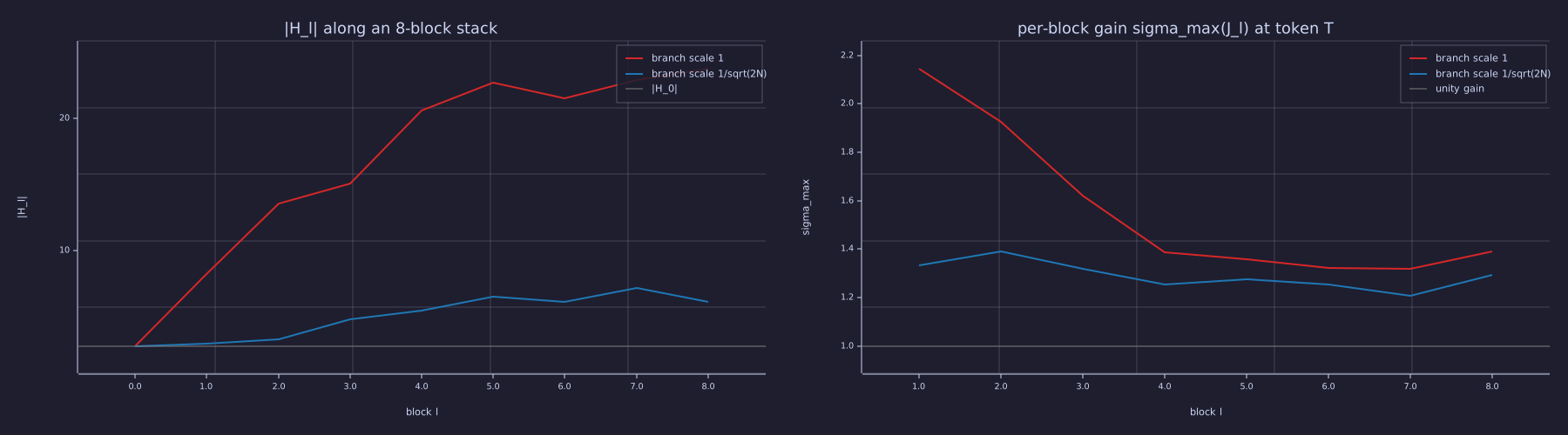
Left: as initialised, eight blocks multiply the stream norm by 4.3; with the \(1/\sqrt{2N}\) branch scaling the same weights give 1.3. Right: the per-block gain starts above 2 for the unscaled stack and settles near 1.3 once the stream is large relative to the branches; the scaled stack sits near 1.3 from the first block. Every block measured here has \(\sigma_{\max}(\mathbf{J}) \ge 1\); the identity path does not guarantee that, but it does pin every singular value of \(\mathbf{J} = \mathbf{I} + \partial f\) into \([\,1 - \|\partial f\|,\; 1 + \|\partial f\|\,]\), so a small branch keeps the block's gain near \(1\) in every direction — the "gradient highway" of Lesson 12 read forwards.
Information
Model. A transformer is a conditional-entropy refinement pipeline. The bigram baseline (Lesson 05) achieves \(H(X_{t+1} \mid X_t)\); a stack of blocks can only do better by extracting information from the longer context, and in the limit of unlimited capacity and data it approaches the true \(H(X_{t+1} \mid X_{1..t})\) of the source. How much each block lowers the achieved conditional entropy is an empirical question — the scaling laws of Lesson 14 — not a fixed amount per layer. The two sublayers play different roles in that pipeline: attention is the only place mutual information between past tokens and the next token can enter row \(t\) (it is the only row-mixing map — the perturbation test); the FFN cannot add information about \(X_{t+1}\) that was not already in row \(t\) (data-processing inequality, Lesson 11) — it re-shapes the row so the next block's attention can extract a different fragment. Multi-head attention splits the extraction into \(H\) parallel channels that share the residual stream and are not, in general, orthogonal (Lesson 09). The residual stream is the lossless backbone (Lesson 12): \(\mathbf{H}_{\text{in}}\) is preserved through H_in + sublayer(LN(H_in)) no matter what the sublayer does.
Exact. Each attention row is a distribution over \(t\) keys, so its entropy is at most \(\log_2 t\) bits; the deficit \(\log_2 t - H(\mathbf{A}_{t,:})\) is how far the head has moved from uniform prefix averaging (Lesson 08's row entropy). At random initialisation the deficits are modest but not zero — head 2 stays near the ceiling, while head 1 already concentrates its weight at \(t = 2\) (the \(0.94\) tap printed under the Signals lens); neither pattern has been learned yet:
bound = log2(1:T);
H_1 = row_entropies_bits(A_1);
H_2 = row_entropies_bits(A_2);
print("log2 t bound (bits):        ", bound);
print("row entropy, head 1 (bits): ", H_1);
print("row entropy, head 2 (bits): ", H_2);
figure();
plot(1:T, bound, "color", "gray", "label", "log2 t (uniform prefix average)")
hold("on")
plot(1:T, H_1, "color", "blue", "label", "head 1")
plot(1:T, H_2, "color", "red", "label", "head 2")
hold("off")
title("attention row entropy vs the uniform bound")
xlabel("query position t")
ylabel("bits")log2 t bound (bits): [1×4] 0.000000 1.000000 1.584963 2.000000
row entropy, head 1 (bits): [1×4] 0.000000 0.328409 1.110058 1.712712
row entropy, head 2 (bits): [1×4] 0.000000 0.910635 1.531749 1.519905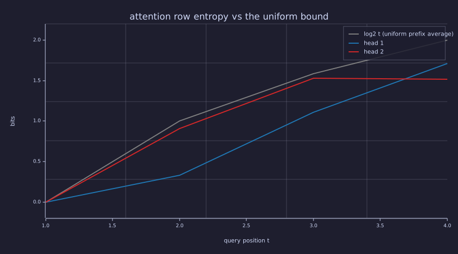
Head 2 sits within half a bit of the \(\log_2 t\) ceiling at every position; head 1 falls \(0.67\) bits short at \(t = 2\) (\(0.33\) of a possible \(1\) bit) and \(0.3\)–\(0.5\) bits short after that. At initialisation the block is still closer to Lesson 07's prefix average than to a routed one, and the routing information (the gap to the grey line) is what training will shape.
Sidebar: Dropout
Theory
Real transformer blocks insert dropout at four points: on the attention probability matrix right after the softmax (GPT-2's attn_pdrop; nanoGPT's self.attn_dropout(att)), after the attention output projection, after the FFN output projection, and on the embedded inputs before the first block. Dropout zeros each activation independently with probability \(p_{\text{drop}}\) during training and scales the survivors by \(1 / (1 - p_{\text{drop}})\) so the expected magnitude is preserved:
\[\tilde a_i = \begin{cases} a_i / (1 - p_{\text{drop}}) & \text{w.p. } 1 - p_{\text{drop}} \\ 0 & \text{w.p. } p_{\text{drop}} \end{cases}\]
At evaluation time dropout is off — the full forward pass runs deterministically. This train-vs-eval split is the most common source of bugs in transformer training code: forgetting to disable dropout at eval inflates the validation loss artificially.
Why it helps
Dropout breaks the model's ability to rely on any specific co-adaptation between activations — every forward pass sees a different random subset of features. It acts as a cheap ensemble (averaging over \(2^{n}\) thinned networks) and is one of the few regularisers cheap enough to compose with everything else in the stack.
nanoGPT uses \(p_{\text{drop}} = 0\) by default (large-scale pretraining is regularised by data) but exposes it as a hyperparameter. Small models, small datasets, and any fine-tune on limited data should turn it on; typical values are \(0.1\) or \(0.2\).
These lessons do not implement dropout in the standalone scripts to keep the forward pass deterministic and verifiable against expected outputs.
Sidebar: Encoder–Decoder and Cross-Attention
Theory
The original Attention Is All You Need architecture is encoder–decoder: two stacks of blocks connected by a third attention type. The encoder reads the source sequence (e.g. an English sentence); the decoder generates the target sequence (e.g. its French translation) one token at a time. The decoder block has three sublayers instead of two:
- Masked self-attention — same as in this lesson, decoder queries attend to past decoder positions only.
- Cross-attention — decoder queries attend to encoder outputs: \(\mathrm{Attn}(Q^{\text{dec}}, K^{\text{enc}}, V^{\text{enc}})\). The Q comes from the decoder, K and V come from the encoder. There is no causal mask on the encoder side — the decoder can attend to the entire source sentence.
- Feed-forward — same as in this lesson.
The encoder block has only the first and third (no cross-attention; no causal mask on its own self-attention).
Why GPT dropped the encoder
For open-ended generation (continue this text) there is no separate "source" sequence — the model conditions on its own past tokens. A decoder-only stack with causal self-attention is sufficient and halves the parameter count for the same depth. Encoder–decoder remains standard for:
- Sequence-to-sequence tasks with a clear input/output split: machine translation, summarisation, speech recognition.
- Models like T5 that frame every task as text-to-text with an explicit source.
The lessons in this series build a decoder-only stack (GPT-style). To convert into an encoder–decoder model, add a sibling stack with no causal mask and insert a cross-attention sublayer between the masked self-attention and the FFN of each decoder block.
Key Takeaways
- The Pre-LN transformer block is
H + MHA(LN(H))followed byH' + FFN(LN(H'))— two residual sublayers around the persistent residual stream. - The block acts on a \(T \times d_{\text{model}}\) signal along two axes: attention is the only operation that mixes rows (time), and causally; LayerNorm and the FFN act per row and mix only columns (channels).
- Tensor shape is \((T, d_{\text{model}})\) at every step of the residual stream; FFN widens to \((T, d_{\text{ff}})\) internally and contracts back. Blocks stack because input and output shapes match.
- Along depth the block is one step of an open-loop nonlinear system \(\mathbf{H}_{\ell+1} = \mathbf{H}_\ell + f_\ell(\mathbf{H}_\ell)\); as initialised the stream norm grows with depth, and the \(1/\sqrt{2N}\) branch scaling holds it near its input scale.
- Per-block parameter count: \(4 d_{\text{model}}^2\) (attention) + \(8 d_{\text{model}}^2\) (FFN) + small bias / LN terms — FFN holds twice the parameters; attention's compute overtakes the FFN's only beyond \(T \approx 4 d_{\text{model}}\) (Lesson 14 computes it).
Standalone Scripts
| Script | What it computes |
|---|---|
block_forward.rlab | one Pre-LN transformer block end-to-end with \(T = 4, d_{\text{model}} = 8, H = 2\); prints shape at every step; signed 1×3 heatmap of \(\mathbf{H}_{\text{in}}\), \(\mathbf{A}_{\text{out}}\), \(\mathbf{F}_{\text{out}}\) |
two_block_stack.rlab | runs the same block twice with different weights; prints residual-stream magnitude after each block |
mixing_axes.rlab | the perturbation test: bump token 3 at each sublayer's input; per-token response sums and a 1×2 signed heatmap |
block_gain_vs_depth.rlab | 2-, 4-, 8-block stacks with and without the \(1/\sqrt{2N}\) branch scaling: \(\lVert \mathbf{H}_\ell \rVert\) and the finite-difference block Jacobian's \(\sigma_{\max}\) and spectral radius |
Run all with make lesson-13 (or rustlab run lessons/13-transformer-block/<name>.rlab).
Expected Numerical Outputs Summary
| Variable | Expected Value |
|---|---|
size(H_in) | [4, 8] |
size(H_norm1) | [4, 8] |
size(A_out) (MHA output) | [4, 8] |
size(F_pre) (FFN hidden) | [4, 32] |
size(F_out) | [4, 8] |
size(H_out) | [4, 8] (= input shape — block is shape-preserving) |
norm(H_in) / norm(H_mid) / norm(H_out) | 6.07 / 9.20 / 10.54 |
norm(A_out) / norm(H_in) | 0.987 |
norm(F_out) / norm(H_mid) | 0.521 |
sum(abs(dA), 2)' / sum(abs(dF), 2)' (responses to a bump at token 3) | [0, 0, 0.775, 0.352] / [0, 0, 1.759, 0]; all 8 channels of row 3 non-zero in dF |
norm(H_out2) (after block 2) | 14.85 |
n_attn (\(d_{\text{model}} = 8\)) | 256 |
n_ffn | 512 |
n_ffn / n_attn | 2 |
n_block | 808 (840 with the two LN affines) |
sum(A_1, 2)' | [1, 1, 1, 1] |
A_1(4, :) | [0.066, 0.210, 0.502, 0.222] |
8-block stack: n_u(9)/n_u(1) vs n_s(9)/n_s(1); max(g_u) vs max(g_s) | 4.26 vs 1.26; 2.14 vs 1.39 |
H_1 (head-1 row entropies, bits) | [0, 0.328, 1.110, 1.713] vs bound [0, 1, 1.585, 2] |
Exercises
- Shape check across configs. Re-run the block with \(T = 16, d_{\text{model}} = 64, H = 8\). List the shape of \(\mathbf{H}_{\text{in}}, \mathbf{H}_{\text{mid}}, \mathbf{H}_{\text{out}}, \mathbf{F}_{\text{pre}}\), \(\mathbf{F}_{\text{out}}\). Which intermediate shapes change with \(H\)? Which don't?
- Without residuals. Remove the two
+operations in the block (just useH_mid = A_outandH_out = F_out). Run two blocks in a row. How does \(\|\mathbf{H}_{\text{out}}\|\) compare to \(\|\mathbf{H}_{\text{in}}\|\)? Connect to Lesson 12's magnitude collapse demo and to the per-block gain plot in the Systems lens — what happens to \(\sigma_{\max}(\mathbf{J})\) without the identity path? - Post-LN variant. Rewrite the block as
H_mid = LN(H_in + MHA(H_in))andH_out = LN(H_mid + FFN(H_mid))(Post-LN). Confirm the final shape is unchanged. Why might this version need a learning-rate warmup that Pre-LN doesn't? - Perturb a different token. Repeat the perturbation test with the bump on token 1 instead of token 3. Which rows of the MHA response are now non-zero, and why is that the maximum spread a causal block allows?
- Bias accounting. Add the LayerNorm affine parameters \((\boldsymbol{\gamma}, \boldsymbol{\beta})\) for both LN1 and LN2 to the count. By how much does the per-block total change? At what \(d_{\text{model}}\) do these become negligible compared to the \(12 d_{\text{model}}^2\) matrix budget?
What's next
Lesson 14 wraps the block into the full GPT decoder: a token embedding (Lesson 04), positional encoding (Lesson 10), \(N\) stacked transformer blocks (this lesson), a final LayerNorm, and a language-modelling head that projects the residual stream to vocabulary logits. It proves end-to-end that the whole model is causal, prints the parameter count and the FLOPs per token of every component for a small GPT config, and confirms the breakdown matches a known reference. After Lesson 14 you have every piece needed to train the architecture — Phase 6 onward fills in the training loop, optimizer, and evaluation.