Lesson 02: Probability & Softmax

A language model produces raw scores called logits — one per vocabulary token. This lesson derives the softmax function that converts logits into a valid probability distribution — it is the maximum-entropy distribution consistent with an expected score, not an arbitrary construction — and introduces the temperature \(\tau\) and entropy as tools for reading model confidence. (Temperature is \(\tau\) throughout this course; \(T\) is reserved for sequence length.)

Learning Objectives

Interpret the output of a language model as a probability distribution over the vocabulary.
Derive softmax as the maximum-entropy distribution under an expected-score constraint, and name the partition function \(Z\) and log-sum-exp.
Read logits as log-odds, and state the softmax Jacobian in one line.
Explain the role of temperature \(\tau\) — the \(\tau \to 0\) and \(\tau \to \infty\) limits — in controlling the sharpness of a distribution.
Compute Shannon entropy in bits and read entropy-versus-\(\tau\) as the model's confidence curve.

Background

One-hot encoding and the unigram entropy from 01-tokens-and-encoding. The exponential and logarithm functions \(e^x\), \(\ln x\), \(\log_2 x\). Lagrange multipliers for a constrained maximum. The definition of a probability distribution: non-negative values that sum to 1.

From Scores to Probabilities

Theory

Logits \(\mathbf{z} = (z_1, \ldots, z_{|\mathcal{V}|})\) can be any real numbers. We want a distribution \(\mathbf{p}\) that (1) is non-negative, (2) sums to 1, and (3) preserves the ordering of the logits. Many maps do that; softmax is the one singled out by a principle.

Derivation — the maximum-entropy distribution. Among all distributions with a prescribed expected score \(\sum_i p_i z_i = \mu\), pick the one that assumes the least: the one with maximum entropy \(H(\mathbf{p}) = -\sum_i p_i \ln p_i\) (nats here; bits differ by the constant \(1/\ln 2\), which does not move the maximiser). With multipliers \(\alpha\) for normalisation and \(\beta\) for the score constraint, the Lagrangian is

\[\mathcal{L}(\mathbf{p}, \alpha, \beta) = -\sum_i p_i \ln p_i + \alpha \Big(\sum_i p_i - 1\Big) + \beta \Big(\sum_i p_i z_i - \mu\Big).\]

\[\frac{\partial \mathcal{L}}{\partial p_i} = -\ln p_i - 1 + \alpha + \beta z_i = 0 \quad\Longrightarrow\quad p_i = e^{\alpha - 1} \, e^{\beta z_i}.\]

Normalisation fixes the first factor, \(e^{\alpha - 1} = 1 / \sum_j e^{\beta z_j}\), so

\[p_i = \frac{e^{\beta z_i}}{Z(\beta)}, \qquad Z(\beta) = \sum_{j=1}^{|\mathcal{V}|} e^{\beta z_j}.\]

\(Z\) is the partition function; \(\beta\) is set by the constraint \(\mu\) and is written \(\beta = 1/\tau\) — the inverse temperature. Because \(-\sum p_i \ln p_i\) is strictly concave and the constraints are linear, this stationary point is the unique maximum. At \(\tau = 1\) it is the standard softmax: \(\mathbf{p} = \text{softmax}(\mathbf{z})\), \(p_i = e^{z_i} / Z\).

Log-sum-exp. \(\ln Z(\mathbf{z}) = \ln \sum_j e^{z_j} \equiv \text{LSE}(\mathbf{z})\), so \(p_i = e^{z_i - \text{LSE}(\mathbf{z})}\) and \(\nabla_{\mathbf{z}} \text{LSE} = \text{softmax}(\mathbf{z})\). LSE is a smooth maximum: \(\max_j z_j \le \text{LSE}(\mathbf{z}) \le \max_j z_j + \ln |\mathcal{V}|\).

Numerical stability

\(\text{LSE}(\mathbf{z}) = m + \text{LSE}(\mathbf{z} - m)\) for any constant \(m\), so implementations subtract \(m = \max(\mathbf{z})\) before exponentiating — the constant \(e^{-m}\) cancels top and bottom, and nothing overflows. The same shift invariance means softmax only sees differences of logits.

Logits are log-odds. Dividing two components, \(\ln \dfrac{p_i}{p_j} = z_i - z_j\): a logit gap of one unit is a factor \(e\) in probability. For two classes, \(p_1 = \dfrac{e^{z_1}}{e^{z_1} + e^{z_2}} = \dfrac{1}{1 + e^{-(z_1 - z_2)}} = \sigma(z_1 - z_2)\) — the logistic sigmoid of the log-odds.

The Jacobian. Differentiating \(p_i = e^{z_i}/Z\) gives, in one line, \(\dfrac{\partial p_i}{\partial z_j} = p_i(\delta_{ij} - p_j)\) — the matrix \(\text{diag}(\mathbf{p}) - \mathbf{p}\mathbf{p}^\top\), whose rows sum to zero (shift invariance again). 03-cross-entropy-loss uses it to reduce the loss gradient to \(\mathbf{p} - \mathbf{y}\).

Example — Softmax, Z, log-sum-exp, and log-odds in numbers

text

z = [2.0, 1.0, 0.5, -0.5];
p = softmax(z);
Z = sum(exp(z));
LSE = log(Z);

print("p = softmax(z):", p, "  sum =", sum(p));
print("Z =", Z, "  LSE = ln Z =", LSE, "  exp(z - LSE) =", exp(z - LSE));
print("shift invariance max|softmax(z + 100) - p| =", max(abs(softmax(z + 100) - p)));
print("log-odds: z1 - z2 =", z(1) - z(2), "  ln(p1/p2) =", log(p(1) / p(2)));

J = diag(p) - p' * p;                    % dp_i/dz_j = p_i (delta_ij - p_j)
print("Jacobian diag(p) - p p':");
print(J);
print("max |row sum of J| (should be 0):", max(max(abs(sum(J, 2)))));

text

p = softmax(z): [1×4]  0.597695  0.219880  0.133364  0.049062   sum = 1
Z = 12.362589857802456   LSE = ln Z = 2.514674965500975   exp(z - LSE) = [1×4]  0.597695  0.219880  0.133364  0.049062
shift invariance max|softmax(z + 100) - p| = 0
log-odds: z1 - z2 = 1   ln(p1/p2) = 1
Jacobian diag(p) - p p':
Matrix(4x4)
  [0.240456, -0.131421, -0.079711, -0.029324]
  [-0.131421, 0.171533, -0.029324, -0.010788]
  [-0.079711, -0.029324, 0.115578, -0.006543]
  [-0.029324, -0.010788, -0.006543, 0.046655]
max |row sum of J| (should be 0): 0.0000000000000000242861286636753

Token 1 gets \(p_1 = 0.598\) of the mass with \(Z = 12.363\) and \(\text{LSE} = 2.515\); adding 100 to every logit changes nothing, and \(z_1 - z_2 = \ln(p_1/p_2) = 1.000\) exactly. The Jacobian's diagonal entry \(p_1(1 - p_1) = 0.240\) is the largest: the most probable token is also the most sensitive to its own logit.

Temperature Scaling

Theory

The temperature \(\tau > 0\) scales the logits before softmax:

\[p_i(\tau) = \frac{e^{z_i / \tau}}{\sum_{j} e^{z_j / \tau}} = \frac{e^{z_i/\tau}}{Z(1/\tau)}.\]

Temperature	Limit	Entropy
\(\tau \to 0\) (cold)	\(z_i/\tau\) gaps grow without bound: all mass on \(\arg\max_i z_i\) — a hard argmax	\(H \to 0\)
\(\tau = 1\) (neutral)	Standard softmax	between
\(\tau \to \infty\) (hot)	\(z_i/\tau \to 0\) for every \(i\): \(p_i \to 1/\lvert\mathcal{V}\rvert\) — uniform	\(H \to \log_2 \lvert\mathcal{V}\rvert\)

Temperature does not change which token has the highest probability — the log-odds \((z_i - z_j)/\tau\) keep their sign — it changes how much higher it is. Temperature is the knob the generation stage (21-sampling-and-generation) uses to trade focused against diverse output.

Example — Softmax of four logits at four temperatures

text

p_cold    = softmax(z / 0.5);
p_neutral = softmax(z / 1.0);
p_warm    = softmax(z / 2.0);
p_hot     = softmax(z / 5.0);

print("tau=0.5 (cold)   :", p_cold);
print("tau=1.0 (neutral):", p_neutral);
print("tau=2.0 (warm)   :", p_warm);
print("tau=5.0 (hot)    :", p_hot);
print("sum at tau=0.5:", sum(p_cold));

text

tau=0.5 (cold)   : [1×4]  0.839025  0.113550  0.041773  0.005653
tau=1.0 (neutral): [1×4]  0.597695  0.219880  0.133364  0.049062
tau=2.0 (warm)   : [1×4]  0.422761  0.256418  0.199698  0.121123
tau=5.0 (hot)    : [1×4]  0.315848  0.258594  0.233986  0.191572
sum at tau=0.5: 1.0000000000000002

Each row sums to 1.000 — a valid distribution. At \(\tau = 0.5\) token 1 gets \(0.839\) of the mass; at \(\tau = 2\) only \(0.423\); at \(\tau = 5\) it is \(0.316\), closing in on the uniform \(0.25\).

Example — PMFs at τ ∈

A PMF over four tokens is four numbers on a 1-based index axis, so it is drawn as stems, not as a curve:

text

figure();
subplot(2, 2, 1)
stem(1:4, p_cold)
title("tau = 0.5 (cold)")
ylim([0, 1])
subplot(2, 2, 2)
stem(1:4, p_neutral)
title("tau = 1.0")
ylim([0, 1])
subplot(2, 2, 3)
stem(1:4, p_warm)
title("tau = 2.0 (warm)")
ylim([0, 1])
subplot(2, 2, 4)
stem(1:4, p_hot)
title("tau = 5.0 (hot): nearly uniform")
ylim([0, 1])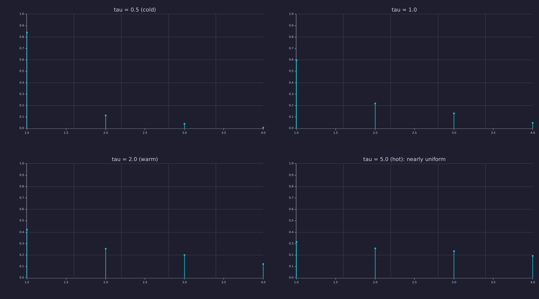

plot 1

Tip

All four panels share the \([0, 1]\) scale. The tallest stem is always token 1 — temperature never reorders — but by \(\tau = 5\) the four stems are within a factor of about 1.65 of each other, heading for the flat \(0.25\) line.

Example — Animation: from argmax to uniform

Sweeping \(\tau\) from \(0.05\) to \(50\) on a log grid morphs the PMF continuously from a single spike (the hard argmax) to the uniform distribution:

text

figure();
taus_anim = logspace(log10(0.05), log10(50), 32);
for k = 1:32
  pk = softmax(z / taus_anim(k));
  stem(1:4, pk)
  title(sprintf("softmax(z / tau),  tau = %.2f", taus_anim(k)))
  ylim([0, 1])
  frame()
end
saveanim("softmax_temperature.gif", 8)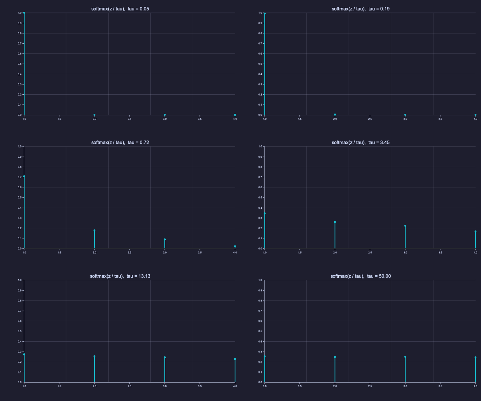

animation 2

Tip

Watch the first stem: it starts at 1.0, passes 0.598 at \(\tau = 1\), and settles toward 0.25. The other three rise in order of their logits and never overtake each other.

Shannon Entropy

Theory

The entropy of a distribution \(\mathbf{p}\) measures how uncertain or spread-out it is:

\[H(\mathbf{p}) = -\sum_{i=1}^{|\mathcal{V}|} p_i \log_2 p_i \quad [\text{bits}], \qquad \text{with the convention } 0 \log 0 = 0.\]

The convention is the limit \(\lim_{p \to 0^+} p \log p = 0\): an outcome of probability zero contributes nothing. Softmax outputs are strictly positive, so the convention is never triggered here; it matters for one-hot targets and for the shared helpers in lib/info.rlab, which implement it by skipping zero entries.

\(H = 0\): all mass on one token (perfectly certain).
\(H = \log_2 |\mathcal{V}|\): uniform distribution (maximally uncertain) — the maximum, by the same Lagrangian as above with the score constraint removed.

Higher temperature \(\to\) higher entropy, monotonically: differentiating the Gibbs form gives \(dH/d\tau = \text{Var}_p(z)/\tau^3 \ge 0\) (in nats), with equality only when all logits tie.

Example — Entropy at four temperatures

Every \(p_i > 0\), so the sum is written directly:

text

vocab_size = 4;
H05 = -sum(p_cold    .* log2(p_cold));
H10 = -sum(p_neutral .* log2(p_neutral));
H20 = -sum(p_warm    .* log2(p_warm));
H50 = -sum(p_hot     .* log2(p_hot));
print("H(tau=0.5) =", H05, " H(tau=1) =", H10, " H(tau=2) =", H20, " H(tau=5) =", H50, "bits");

text

H(tau=0.5) = 0.8024252882978413  H(tau=1) = 1.525296073088579  H(tau=2) = 1.8615588961498242  H(tau=5) = 1.9767728958188087 bits

Entropy climbs with temperature: \(H(\tau{=}0.5) = 0.802\), \(H(\tau{=}1) = 1.525\), \(H(\tau{=}2) = 1.862\), \(H(\tau{=}5) = 1.977\) bits, against a maximum of \(\log_2 4 = 2\).

Example — Sanity checks: uniform vs. near-deterministic

text

p_uniform = ones(vocab_size) / vocab_size;
H_uniform = -sum(p_uniform .* log2(p_uniform));

p_det = [0.999, 0.0003, 0.0003, 0.0004];
H_det = -sum(p_det .* log2(p_det));
print("H(uniform) =", H_uniform, "bits   H(near-deterministic) =", H_det, "bits");

text

H(uniform) = 2 bits   H(near-deterministic) = 0.012978708331915804 bits

Uniform over 4 tokens: \(H = 2.000\) bits (matches \(\log_2 4 = 2\)). Near-deterministic: \(H = 0.0130\) bits. From here on the lesson calls entropy_bits from lib/info.rlab — the same sum, with the \(0 \log 0 = 0\) convention built in.

Engineering Lenses

No systems reading adds to this lesson: softmax is a memoryless map with no state and no update law. The statistical-mechanics reading of the Boltzmann form is an information statement and sits under Information.

Signals

Exact. Softmax is a soft-argmax: \(\tau \to 0\) recovers the hard comparator \(\arg\max\), and every finite \(\tau\) returns a graded decision instead of a hard one. For two hypotheses with log-likelihoods (plus log-priors) \(z_1, z_2\), the posterior is \(\text{softmax}(\mathbf{z})\) and \(\Lambda = z_1 - z_2\) is the log-likelihood ratio; the two-class softmax \(p_1 = \sigma(\Lambda/\tau)\) is a soft-decision demapper — the block that feeds a soft-input decoder — where a hard detector would output \(\text{sign}(\Lambda)\). For BPSK in Gaussian noise \(\Lambda = 2Ay/\sigma^2\), so dividing \(\Lambda\) by \(\tau\) is the same operation as multiplying the noise variance by \(\tau\): temperature enters exactly where noise variance does.

text

z2 = [2.0, 1.0];                                  % two classes, LLR = 1
for tau = [0.5, 1.0, 2.0]
  p_sm = softmax(z2 / tau);
  print("tau =", tau, ": softmax(z/tau)(1) =", p_sm(1), "  sigma(LLR/tau) =", 1 / (1 + exp(-(z2(1) - z2(2)) / tau)));
end

Lam = linspace(-6, 6, 121);
figure();
plot(Lam, 1 ./ (1 + exp(-Lam / 0.5)), "color", "blue",  "label", "tau = 0.5")
hold("on")
plot(Lam, 1 ./ (1 + exp(-Lam / 1.0)), "color", "green", "label", "tau = 1")
plot(Lam, 1 ./ (1 + exp(-Lam / 2.0)), "color", "red",   "label", "tau = 2")
hline(0.5, "gray", "hard decision threshold")
hold("off")
title("Soft decision p_1 = sigma(LLR / tau)")
xlabel("log-likelihood ratio  LLR = z_1 - z_2")
ylabel("p_1")

text

tau = 0.5 : softmax(z/tau)(1) = 0.8807970779778823   sigma(LLR/tau) = 0.8807970779778823
tau = 1 : softmax(z/tau)(1) = 0.7310585786300049   sigma(LLR/tau) = 0.7310585786300049
tau = 2 : softmax(z/tau)(1) = 0.6224593312018546   sigma(LLR/tau) = 0.6224593312018546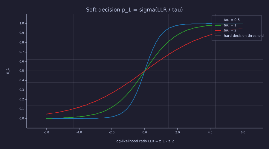

plot 3

Tip

All three curves cross \(p_1 = 0.5\) at \(\text{LLR} = 0\) — the hard decision never moves. Lower \(\tau\) steepens the curve toward the sign function; higher \(\tau\) flattens it toward \(0.5\) everywhere, exactly what more noise does to a demapper.

Information

Exact. Softmax is the maximum-entropy distribution under the expected-score constraint — the derivation above — and the claim can be checked numerically. The direction \(\mathbf{v} = (1, -1, -1, 1)\) changes neither the total mass (\(\sum v_i = 0\)) nor the expected score (\(\sum v_i z_i = 0\) for this \(\mathbf{z}\)), so \(\mathbf{p} \pm \varepsilon \mathbf{v}\) satisfies the same constraints as \(\mathbf{p} = \text{softmax}(\mathbf{z})\) and must have lower entropy:

text

v = [1, -1, -1, 1];
mu = sum(p .* z);
q_plus  = p + 0.03 * v;
q_minus = p - 0.03 * v;
print("constraint check: sum(v) =", sum(v), "  sum(v .* z) =", sum(v .* z), "  E_q[z] =", sum(q_plus .* z), " = mu =", mu);
print("H(p) =", entropy_bits(p), "  H(p + 0.03 v) =", entropy_bits(q_plus), "  H(p - 0.03 v) =", entropy_bits(q_minus), "bits");

text

constraint check: sum(v) = 0   sum(v .* z) = 0   E_q[z] = 1.4574202929204703  = mu = 1.4574202929204705
H(p) = 1.525296073088579   H(p + 0.03 v) = 1.5047064047570426   H(p - 0.03 v) = 1.499543090911674 bits

Both perturbed distributions lose entropy — \(1.5047\) and \(1.4995\) bits against \(1.5253\) — while keeping \(\mathbb{E}[z] = 1.457\): softmax is the least-committed distribution consistent with the logits.

Exact. Entropy is a continuous, monotone function of temperature with the two limits derived above. Sweeping \(\tau\) on a log axis shows both asymptotes at once:

text

taus = logspace(log10(0.05), log10(50), 60);
H_tau = zeros(length(taus));
for k = 1:length(taus)
  H_tau(k) = entropy_bits(softmax(z / taus(k)));
end
print("H at tau = 0.05:", H_tau(1), " bits;  at tau = 50:", H_tau(end), " bits");

figure();
semilogx(taus, H_tau, "color", "blue", "label", "H(softmax(z / tau))")
hold("on")
yline(log2(vocab_size), "red", "log2|V| = 2 (uniform)")
yline(0, "gray", "0 (argmax)")
hold("off")
title("Entropy vs temperature")
xlabel("tau (log axis)")
ylabel("H  [bits]")

text

H at tau = 0.05: 0.00000006245012320586353  bits;  at tau = 50: 1.9997655839197161  bits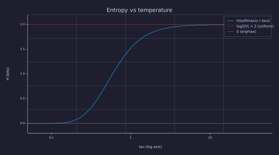

plot 4

Tip

The curve is an S between the two reference lines: flat near 0 bits for \(\tau \lesssim 0.1\) (a hard argmax), steepest around \(\tau \approx 0.5\)–\(1\), and within \(0.001\) bits of \(\log_2 4 = 2\) by \(\tau = 50\). The four entropies computed above are four points on this curve.

Exact. The form \(p_i = e^{z_i/\tau}/Z\) is the Boltzmann–Gibbs distribution of statistical mechanics with \(z_i = -E_i\) (negative energies), \(\tau\) the temperature, and \(Z\) the partition function; the name is not a metaphor — as \(\tau \to 0\) the system freezes into its ground state (highest logit), and \(\ln Z\) is the free-energy generating function whose gradient is the mean occupancy \(\mathbf{p}\). And \(H(\mathbf{p})\) is the source-coding bound: the minimum expected code length for symbols drawn from \(\mathbf{p}\) is \(H\) bits, with the optimal code giving symbol \(i\) a length of \(-\log_2 p_i\) bits. The entropies computed above are therefore bit-budgets:

Distribution	\(H\) (bits)	Optimal avg bits/token
`p_cold` (\(\tau{=}0.5\))	\(0.802\)	\(0.802\)
`p_neutral` (\(\tau{=}1\))	\(1.525\)	\(1.525\)
`p_uniform` (4 tokens)	\(2.0\) (= \(\log_2 4\))	\(2.0\) — fixed-width is already optimal

These facts return in 03-cross-entropy-loss (cross-entropy as expected code length under the model) and 20-perplexity-and-evaluation (perplexity as \(2^H\)).

Key Takeaways

Softmax is not a convention: it is the unique maximum-entropy distribution with a prescribed expected score, \(p_i = e^{z_i/\tau} / Z\), with partition function \(Z\) and \(\ln Z = \text{LSE}(\mathbf{z})\).
Logits are log-odds: \(z_i - z_j = \ln(p_i/p_j)\); two classes give the logistic sigmoid; the Jacobian is \(p_i(\delta_{ij} - p_j)\).
Temperature \(\tau\) rescales the log-odds: \(\tau \to 0\) is the hard argmax (\(H \to 0\)), \(\tau \to \infty\) is uniform (\(H \to \log_2|\mathcal{V}|\)), and the ordering never changes.
Entropy in bits is the source-coding bound; softmax with temperature is the Boltzmann distribution and a soft-decision demapper. ML borrowed all three names exactly.

Standalone Scripts

Script	What it computes
`softmax_maxent.rlab`	softmax of `[2.0, 1.0, 0.5, -0.5]`, \(Z\), log-sum-exp, shift invariance, log-odds, the Jacobian, the two-class sigmoid identity, and the max-entropy perturbation check
`softmax_temperature.rlab`	softmax at \(\tau = 0.5, 1, 2, 5\); the 2×2 stem-plot figure
`softmax_animation.rlab`	the argmax-to-uniform GIF over 32 temperatures (`softmax_temperature.gif`)
`entropy.rlab`	entropy at the four temperatures plus uniform and near-deterministic baselines; the entropy-vs-\(\tau\) `semilogx` curve

Run all with make lesson-02 (or rustlab run lessons/02-probability-and-softmax/<name>.rlab).

Expected Numerical Outputs Summary

Variable	Expected Value
`p(1)` (τ = 1)	≈ `0.598`
`Z`, `LSE`	≈ `12.363`, `2.515`
`z(1) - z(2)` = `log(p(1)/p(2))`	`1.000`
`J(1, 1)` = \(p_1(1 - p_1)\)	≈ `0.240`; every row of `J` sums to 0
`p_cold(1)`, `p_warm(1)`, `p_hot(1)`	≈ `0.839`, `0.423`, `0.316`
`H05`, `H10`, `H20`, `H50`	≈ `0.802`, `1.525`, `1.862`, `1.977` bits
`H_uniform`, `H_det`	`2.0`, ≈ `0.013` bits
`softmax(z2 / tau)(1)` at τ = 0.5, 1, 2	≈ `0.881`, `0.731`, `0.622` (= σ(2), σ(1), σ(0.5))
`entropy_bits(q_plus)`, `entropy_bits(q_minus)`	both below `H10` = `1.525` bits
`H_tau(1)`, `H_tau(end)`	≈ `6e-8`, `1.9998` bits

Exercises

Softmax invariance to shift. Show algebraically that adding a constant \(c\) to all logits does not change the softmax output, and relate it to the row sums of the Jacobian. Verify numerically on [2, 1, 0] and [5, 4, 3].
Temperature limits. Write out \(\lim_{\tau \to 0} \text{softmax}(\mathbf{z}/\tau)\) and \(\lim_{\tau \to \infty} \text{softmax}(\mathbf{z}/\tau)\) from the formula, then read both off the entropy-vs-\(\tau\) curve. What happens at \(\tau \to 0\) when two logits tie?
Entropy calculation. For the logits [3.0, 3.0, 3.0, 3.0], compute the softmax probabilities and the entropy by hand. Does the result match \(\log_2 4\)?
Solve for β. In the max-entropy derivation \(\beta\) is fixed by the constraint \(\mu\). For \(\mathbf{z} = [2, 1, 0.5, -0.5]\), find numerically the \(\tau = 1/\beta\) that gives \(\mathbb{E}_p[z] = 1.0\) (bisection on \(\tau \in [0.1, 10]\) is enough). Is it hotter or colder than \(\tau = 1\)?
Softmax Jacobian. Starting from \(p_i = e^{z_i}/Z\), derive \(\partial p_i / \partial z_j = p_i(\delta_{ij} - p_j)\) and show that \(\sum_j \partial p_i / \partial z_j = 0\).

Solution

For \(j = i\): \(\dfrac{\partial}{\partial z_i}\dfrac{e^{z_i}}{Z} = \dfrac{e^{z_i}}{Z} - \dfrac{e^{z_i}\, e^{z_i}}{Z^2} = p_i - p_i^2 = p_i(1 - p_i)\), using \(\partial Z / \partial z_i = e^{z_i}\). For \(j \ne i\): \(\dfrac{\partial}{\partial z_j}\dfrac{e^{z_i}}{Z} = -\dfrac{e^{z_i}\, e^{z_j}}{Z^2} = -p_i p_j\). Both cases read \(p_i(\delta_{ij} - p_j)\). Summing over \(j\): \(p_i\big(1 - \sum_j p_j\big) = p_i(1 - 1) = 0\) — a uniform shift of every logit leaves \(\mathbf{p}\) unchanged, which is exercise 1 seen from the derivative side.

What's next

03-cross-entropy-loss introduces cross-entropy loss — the standard training objective for a language model. Cross-entropy measures the gap between the predicted distribution \(\mathbf{p}\) from this lesson and the one-hot target from Lesson 01; written as \(-z_c + \text{LSE}(\mathbf{z})\) and differentiated with the Jacobian above, its gradient is the bounded error signal \(\mathbf{p} - \mathbf{y}\).