Lesson 07: Context and Naive Averaging
The bigram model (05-bigram-language-model) predicts the next token from a single previous token. That's a structural limit — no amount of data can make it context-aware. Fixing this means letting the prediction depend on all earlier tokens. The simplest aggregator is the prefix average. Writing it as a matrix multiply is the bridge to attention (08-scaled-dot-product-attention); reading that multiply as a causal filter along the token axis is the frame the rest of the course keeps.
Learning Objectives
- Explain why a bigram (Markov-1) language model is context-free beyond a single previous token, and measure that failure in bits.
- Define prefix averaging — the simplest context-aware aggregation — as \(\bar{\mathbf{x}}_t = \frac{1}{t}\sum_{i=1}^{t} \mathbf{x}_i\).
- Rewrite that sum as a matrix multiplication \(\bar{\mathbf{X}} = \mathbf{W}\mathbf{X}\) where \(\mathbf{W}\) is a lower-triangular averaging matrix, and read it as a causal, time-varying FIR filter.
- Read the lower-triangular causal structure of \(\mathbf{W}\) and explain why it enforces the "no peek at the future" rule.
- Articulate the remaining weaknesses of uniform averaging — every past token gets equal weight, and order is lost — that motivate attention (Lesson 08).
Background
Bigram language models, row-normalised probability matrices and the entropy chain rule from 05-bigram-language-model. Linear layers and matrix multiplication from 06-linear-layers-and-gradient-descent. Embeddings as dense row vectors from 04-embeddings-and-similarity. The Engineering Lenses assume you have met a moving-average (FIR) filter and a one-pole (IIR) low-pass and their frequency responses. Notation follows 00-the-llm-as-a-system: tokens are rows (time \(t\)), features are columns.
Where the Bigram Fails
Theory
Consider two sentences sharing an ambiguous token:
river bank watermoney bank safe
bank is the same token in both, but its continuation depends on the history. A bigram sees only the previous token, so both histories collapse to the same row of \(\mathbf{P}\).
Example — P(next | bank) collapses to a 50/50
vocab_size = 5;
% river=1, bank=2, water=3, money=4, safe=5

C = zeros(vocab_size, vocab_size);
C(1, 2) = 1;   % river -> bank
C(2, 3) = 1;   % bank  -> water
C(4, 2) = 1;   % money -> bank
C(2, 5) = 1;   % bank  -> safe

P = zeros(vocab_size, vocab_size);
for i = 1:vocab_size
  row_sum = sum(C(i, :));
  if row_sum > 0
    P(i, :) = C(i, :) / row_sum;
  end
end

p_after_bank = P(2, :);
The bigram's continuation distribution after bank is
\[P(\text{next} \mid \text{bank}) = [0, 0, 0.5, 0, 0.5].\]
P(water | bank) = \(0.50\), P(safe | bank) = \(0.50\) — whether the history was river bank or money bank. The model has no mechanism to tell them apart.
Example — Bar of P(next | bank)
figure();
labels = {"river", "bank", "water", "money", "safe"};
bar(labels, p_after_bank)
title("P(next | bank) — identical regardless of prior context")
ylabel("Probability")
ylim([0, 1])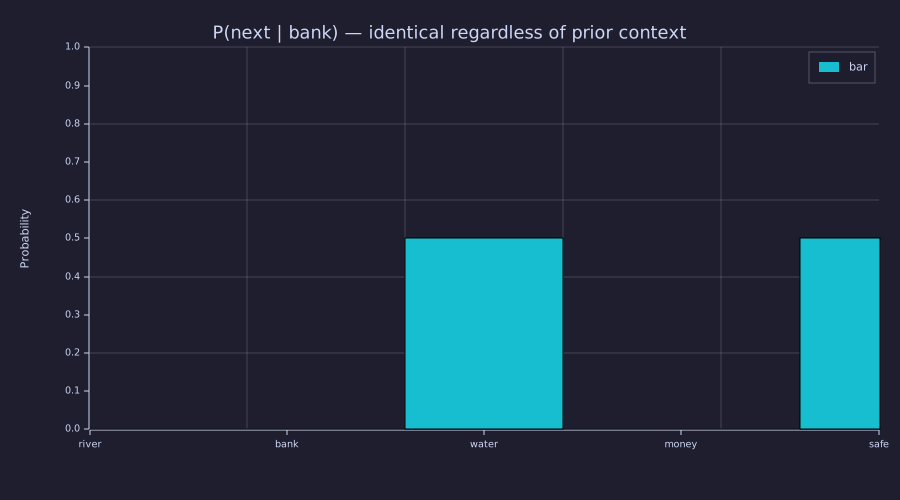
Two equal bars: one full bit of uncertainty that the earlier token (river or money) would have removed. The Information lens below puts a number on it.
This is a structural failure, not a data failure.
The Fix: Summarise the Whole Prefix
Theory
If the prediction depends only on the last token, it can't see prior context. So let the state at position \(t\) summarise every earlier token. The simplest summary is the average
\[\bar{\mathbf{x}}_t \;=\; \frac{1}{t}\sum_{i=1}^{t} \mathbf{x}_i.\]
Each \(\bar{\mathbf{x}}_t\) is a "bag of past tokens" — every prior embedding blended in with equal weight.
Rewrite as a Matrix Multiply
Theory
Stack embeddings into \(\mathbf{X} \in \mathbb{R}^{T \times d}\) and define a lower-triangular averaging matrix \(\mathbf{W}\):
\[\mathbf{W}_{t, i} = \begin{cases} \frac{1}{t} & i \le t \\ 0 & i > t. \end{cases}\]
Then the entire stack of prefix averages is a single matrix multiply
\[\bar{\mathbf{X}} \;=\; \mathbf{W}\mathbf{X}.\]
The upper triangle is zero — this is the causal constraint: position \(t\) cannot see a future token. (In the course notation this \(\mathbf{W}\) is the mixing matrix \(\mathbf{A}\) of 08-scaled-dot-product-attention in its uniform special case; from Lesson 08 on, \(\mathbf{W}\) denotes a learned projection.)
Example — Build W and the input embeddings X
T = 6;
d = 4;

% Rows 1-4 are the one-hot basis; row 5 = x1 + x2 and row 6 = x3 + x4,
% so the averages can be checked by hand.
X = [ 1.0, 0.0, 0.0, 0.0;
      0.0, 1.0, 0.0, 0.0;
      0.0, 0.0, 1.0, 0.0;
      0.0, 0.0, 0.0, 1.0;
      1.0, 1.0, 0.0, 0.0;
      0.0, 0.0, 1.0, 1.0 ];

W = zeros(T, T);                                 % (a) the definition, cell by cell
for t = 1:T
  for i = 1:t
    W(t, i) = 1.0 / t;
  end
end
W_vec  = cumsum(eye(T), 1) ./ repmat((1:T)', 1, T);   % (b) mask [i <= t] divided by the row index t
diff_W = max(reshape(abs(W - W_vec), 1, T * T));
print("max|W_loop - W_vec| =", diff_W);max|W_loop - W_vec| = 0Form (b) mirrors the math \(W_{t, i} = \frac{1}{t} \cdot [i \le t]\): cumsum(eye(T), 1) extends each diagonal 1 down its column (the causal mask), and dividing by the row index sets the weight. It generalises at once — another mask, or another per-row weighting, as the Engineering Lenses do below. (The running-sum loop that the multiply replaces appears in the Systems lens.)
Example — Read X̄ back by hand
X_bar_mm = W * X;
x_bar_3_expected = [1/3, 1/3, 1/3, 0];
err_row3 = max(abs(X_bar_mm(3, :) - x_bar_3_expected));
print("x_bar_3 =", X_bar_mm(3, :), "  max|error| =", err_row3);
print("x_bar_6 =", X_bar_mm(6, :));x_bar_3 = [1×4] 0.333333 0.333333 0.333333 0.000000 max|error| = 0
x_bar_6 = [1×4] 0.333333 0.333333 0.333333 0.333333Row 3 is \((\mathbf{x}_1 + \mathbf{x}_2 + \mathbf{x}_3)/3 = [\tfrac13, \tfrac13, \tfrac13, 0]\) (error \(0.0e+00\)). Row 6 is more telling: rows 5 and 6 of \(\mathbf{X}\) were \(\mathbf{x}_1 + \mathbf{x}_2\) and \(\mathbf{x}_3 + \mathbf{x}_4\), so the six rows sum to \([2, 2, 2, 2]\) and \(\bar{\mathbf{x}}_6 = [\tfrac13, \tfrac13, \tfrac13, \tfrac13]\) — perfectly flat. From \(\bar{\mathbf{x}}_6\) alone you cannot tell which token came last, or that token 6 was x3+x4 rather than x1+x2. The average has kept the set of features and thrown away order and salience.
Example — X, W and X̄ side by side
positions = {"t1", "t2", "t3", "t4", "t5", "t6"};
dims = {"d1", "d2", "d3", "d4"};

figure();
subplot(1, 3, 1)
heatmap(dims, positions, X, "Input X (rows: tokens, cols: features)", "viridis")
subplot(1, 3, 2)
heatmap(positions, positions, W, "W (rows: output time t, cols: input time i)", "viridis")
subplot(1, 3, 3)
heatmap(dims, positions, X_bar_mm, "Prefix averages X_bar = W X", "viridis")
Left to right: sharp one-hot rows; the causal triangle whose row \(t\) is \(t\) equal cells of \(1/t\); and the blurred result whose last row is a single flat colour.
The Remaining Weakness
Theory
Uniform \(1/t\) weights treat every past token as equally informative, and the average is order-blind: any permutation of the first \(t\) tokens gives the same \(\bar{\mathbf{x}}_t\). In "the cat sat on the mat, it was soft", the model standing at was must predict $X_{t+1} = $ soft; the token that tells it what it refers to is mat, several positions back, while the, on and the comma tell it essentially nothing.
Information-theoretic framing. Let \(X_{t+1}\) be the next token and \(X_{1..t}\) the prefix — the same target every later lesson uses. By the chain rule of entropy from 05-bigram-language-model, \(H(X_{t+1} \mid X_t) \ge H(X_{t+1} \mid X_{1..t})\): extra context never hurts, and the gap is the conditional mutual information \(I(X_{t+1};\, X_{1..t-1} \mid X_t)\) — bits about the next token that live further back than one position. Those bits are spread very unevenly over the prefix: \(I(X_{t+1};\, X_i \mid X_{i+1..t})\) is large for \(i = $ `mat` and near zero for $i = $ `the`. A uniform average cannot exploit that unevenness — it dilutes the informative token by $1/t\) along with everything else.
That is exactly what attention does. It replaces the fixed \(1/t\) entries of \(\mathbf{W}\) with \(\mathrm{softmax}(\text{scores})\), where the scores depend on query and key vectors derived from the embeddings themselves — so the model can route weight toward whichever past tokens carry the most information about the next. The lower-triangular (causal) structure and the per-row weighted sum stay identical.
Engineering Lenses
Signals
Exact. \(\bar{\mathbf{X}} = \mathbf{W}\mathbf{X}\) is a causal, linear, time-varying FIR filter along the token axis. Output time \(t\) is \(\bar{\mathbf{x}}_t = \sum_{i \le t} h_t[t - i]\, \mathbf{x}_i\) with taps \(h_t[n] = W_{t,\,t-n}\): row \(t\) of \(\mathbf{W}\) is the impulse response observed at output time \(t\) — a box of \(t\) taps of height \(1/t\). The filter acts on each of the \(d\) feature columns independently, so it is \(d\) identical channels.
figure();
rows_to_show = [2, 4, 6];
for k = 1:3
  t = rows_to_show(k);
  subplot(1, 3, k)
  stem(1:T, W(t, :))
  title(sprintf("row %d of W: %d taps of 1/%d", t, t, t))
  xlabel("input time i")
  ylim([0, 0.6])
end
The box grows with \(t\) and its height falls as \(1/t\): the window never forgets, and each new token gets a smaller share. Time-varying because the impulse response at time 6 is not the one at time 2.
Exact. The exponential moving average \(y_t = \gamma\, y_{t-1} + (1 - \gamma)\, x_t\) is a first-order IIR filter with one pole at \(z = \gamma\) and impulse response \((1-\gamma)\gamma^{n}\), \(n \ge 0\). Renormalised over the tokens available at time \(t\) it is another causal mixing matrix, \(W^{\text{ema}}_{t,i} = (1 - \gamma)\gamma^{t-i} / (1 - \gamma^{t})\) for \(i \le t\) — same triangle, geometric rows instead of flat ones. The box forgets nothing; the EMA forgets with time constant \(-1/\ln\gamma\) tokens.
gamma = 0.8;
W_ema = zeros(T, T);
for t = 1:T
  for i = 1:t
    W_ema(t, i) = (1 - gamma) * gamma ^ (t - i) / (1 - gamma ^ t);
  end
end
tau_ema = -1 / log(gamma);
print("W     row 6 =", W(6, :));
print("W_ema row 6 =", W_ema(6, :), "  (sums to", sum(W_ema(6, :)), ")");
print("EMA pole z = gamma =", gamma, " time constant =", tau_ema, "tokens");W row 6 = [1×6] 0.166667 0.166667 0.166667 0.166667 0.166667 0.166667
W_ema row 6 = [1×6] 0.088819 0.111024 0.138780 0.173476 0.216844 0.271056 (sums to 1.0000000000000002 )
EMA pole z = gamma = 0.8 time constant = 4.481420117724551 tokensModel. Freeze the window at \(t = T\) and the row becomes an LTI filter with a frequency response — "smoother" means low-pass. Frequency is in cycles per token (Nyquist \(= 0.5\)): a feature that flips sign every token is at \(0.5\), a topic that persists for a paragraph is near DC. freqz of the \(T\)-tap box against the EMA (its impulse response truncated at 64 taps, \(\gamma^{64} < 10^{-6}\)):
n_f = 256;
h_box = ones(1, T) / T;                        % row T of W: a T-tap box
h_ema = (1 - gamma) * gamma .^ (0:63);         % one-pole IIR, truncated
R_box = freqz(h_box, n_f, 1.0);                % row 1: f (cycles/token), row 2: H(f) complex
R_ema = freqz(h_ema, n_f, 1.0);
f = real(R_box(1, :));
H_box = abs(R_box(2, :));
H_ema = abs(R_ema(2, :));
print("box first null at 1/T =", 1 / T, "   EMA gain at Nyquist (1-g)/(1+g) =", (1 - gamma) / (1 + gamma), " measured", H_ema(end));

figure();
plot(f, H_box, "color", "blue", "label", "6-tap box")
hold("on")
plot(f, H_ema, "color", "red", "label", "EMA, gamma = 0.8")
hline(1 / sqrt(2), "gray", "-3 dB")
hold("off")
title("|H(f)| — both pass DC with unit gain")
xlabel("frequency (cycles / token)")
ylabel("|H(f)|")
legend("6-tap box", "EMA, gamma = 0.8", "-3 dB")box first null at 1/T = 0.16666666666666666 EMA gain at Nyquist (1-g)/(1+g) = 0.11111111111111108 measured 0.1111131276434191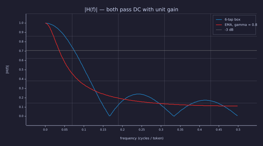
Both curves start at 1 (rows sum to 1, so DC passes unchanged). The box has nulls at multiples of \(1/6\) and sidelobes between them — a sinc; the EMA rolls off monotonically and never gets below \((1-\gamma)/(1+\gamma) = 0.11\). The box crosses −3 dB later than the EMA: the 6-token box is the sharper, but leakier, low-pass.
Analogy. Attention (08-scaled-dot-product-attention) keeps this FIR form but computes the taps from the signal itself — an adaptive filter in spirit, though with no error-driven tap update at inference time.
Systems
Exact. The running mean is a first-order system: \(\bar{\mathbf{x}}_t = \bar{\mathbf{x}}_{t-1} + \tfrac{1}{t}\,(\mathbf{x}_t - \bar{\mathbf{x}}_{t-1})\) (multiply the definition by \(t\) and subtract the \(t-1\) case). Its gain \(1/t\) decays to zero, so the state responds less and less to new input — token 100 moves the average by 1 %. The EMA is the same recursion with constant gain \(1 - \gamma\): fixed pole, fixed memory. 16-adamw-optimizer reuses exactly this one-pole system on gradients.
X_bar_rec = zeros(T, d);
x_bar = zeros(1, d);
for t = 1:T
  x_bar = x_bar + (X(t, :) - x_bar) / t;       % state update with gain 1/t
  X_bar_rec(t, :) = x_bar;
end
diff_rec = max(reshape(abs(X_bar_rec - X_bar_mm), 1, T * d));
print("max|recursion - W*X| =", diff_rec);
print("running-mean gains 1/t:", 1 ./ (1:T), " EMA gain 1 - gamma:", 1 - gamma);max|recursion - W*X| = 0.00000000000000005551115123125783
running-mean gains 1/t: [1×6] 1.000000 0.500000 0.333333 0.250000 0.200000 0.166667 EMA gain 1 - gamma: 0.19999999999999996Information
Exact. Conditioning cannot increase entropy, so \(H(X_{t+1} \mid X_t) \ge H(X_{t+1} \mid X_{1..t})\), and the difference is the bits a longer context recovers. On the two-sentence corpus both sides are computable by the chain rule \(H(X_{t+1} \mid \text{ctx}) = H(\text{ctx}, X_{t+1}) - H(\text{ctx})\) with empirical distributions (the helper below builds them; entropy_bits is from lib/info.rlab).
function H = empirical_entropy_bits(labels)
  % entropy (bits) of the empirical distribution of a vector of integer labels
  counts = zeros(max(labels));
  for m = 1:length(labels)
    counts(labels(m)) = counts(labels(m)) + 1;
  end
  H = entropy_bits(counts / sum(counts));
end

sents = [1, 2, 3;      % river bank water
         4, 2, 5];     % money bank safe
base = vocab_size + 1;
prev = []; ctx = []; nxt = [];
for s = 1:2
  for t = 1:2
    prev = [prev, sents(s, t)];                             % bigram context: last token only
    ctx  = [ctx, sents(s, 1:t) * (base .^ (0:t-1))'];      % full-prefix context, as one integer id
    nxt  = [nxt, sents(s, t + 1)];
  end
end
H_bank   = entropy_bits(P(2, :));
H_bigram = empirical_entropy_bits(prev + base * nxt) - empirical_entropy_bits(prev);
H_prefix = empirical_entropy_bits(ctx + base ^ 3 * nxt) - empirical_entropy_bits(ctx);
print("H(next | bank)               =", H_bank, "bits");
print("H(X_{t+1} | X_t)             =", H_bigram, "bits  (average over the corpus)");
print("H(X_{t+1} | X_{1..t})        =", H_prefix, "bits");
print("I(X_{t+1}; X_{1..t-1} | X_t) =", H_bigram - H_prefix, "bits recovered by the prefix");
order_bits_6 = log2(prod(1:6));
print("order bits a bag of 6 distinct tokens discards: log2(6!) =", order_bits_6);H(next | bank) = 1 bits
H(X_{t+1} | X_t) = 0.5 bits (average over the corpus)
H(X_{t+1} | X_{1..t}) = 0 bits
I(X_{t+1}; X_{1..t-1} | X_t) = 0.5 bits recovered by the prefix
order bits a bag of 6 distinct tokens discards: log2(6!) = 9.491853096329674After bank the bigram is left with \(1.0\) bit; averaged over every position it is \(0.50\) bits per token, and the full prefix drives it to \(0.0\) — every sentence is determined by its first token. The \(0.50\)-bit gap is the floor difference between the Lesson 05 model class and any context-aware one on this corpus; 08-scaled-dot-product-attention measures, row by row, how much of a prefix an attention head actually uses.
Exact. The prefix average is permutation-invariant, so at position \(t\) it also discards the \(\log_2 t!\) bits that distinguish the orderings of \(t\) distinct tokens — \(9.49\) bits at \(t = 6\). 10-positional-encoding puts them back.
Key Takeaways
- A bigram's next-token distribution depends only on the previous token; histories that share the same last token are indistinguishable — on the toy corpus that costs 0.5 bits per token.
- The simplest context-aware summary is a prefix average over all tokens \(1..t\); it is a single matrix multiply \(\bar{\mathbf{X}} = \mathbf{W}\mathbf{X}\) with \(\mathbf{W}\) lower-triangular and each row normalised to sum to 1.
- \(\mathbf{W}\) is a causal, time-varying FIR filter along the token axis — a growing box, hence a low-pass; the EMA is its one-pole IIR cousin, and both have a one-line recursive state update.
- The lower-triangular shape encodes causality — position \(t\) cannot look at the future.
- Uniform averaging discards which past tokens matter and in what order — the next lesson replaces the fixed taps with data-dependent ones.
Standalone Scripts
| Script | What it computes |
|---|---|
context_failure.rlab | bigram count + probability matrix on the bank corpus; bar of \(P(\text{next} \mid \text{bank})\) |
prefix_averaging.rlab | prefix averages two ways (running-sum loop and matrix multiply); hand read-back of rows 3 and 6; labelled heatmaps of \(\mathbf{X}\), \(\mathbf{W}\), \(\bar{\mathbf{X}}\) |
averaging_as_fir.rlab | rows of \(\mathbf{W}\) as impulse responses; the EMA mixing matrix; recursive updates; freqz of the box vs the one-pole IIR |
context_entropy.rlab | \(H(X_{t+1} \mid X_t)\) vs \(H(X_{t+1} \mid X_{1..t})\) on the corpus via the chain rule; the order bits a bag of tokens discards |
Run all with make lesson-07 (or rustlab run lessons/07-context-and-naive-averaging/<name>.rlab).
Expected Numerical Outputs Summary
| Variable | Expected Value |
|---|---|
p_after_bank(3) (\(P(\text{water}\mid\text{bank})\)) | 0.50 |
p_after_bank(5) (\(P(\text{safe}\mid\text{bank})\)) | 0.50 |
W(1, 1); W(2, 1), W(2, 2); W(t, i), \(i \le t\); W(t, i), \(i > t\) | 1.0; 0.5 each; 1/t; 0 |
diff_W, diff_rec (loop vs vectorised \(\mathbf{W}\); recursion vs \(\mathbf{W}\mathbf{X}\)) | 0 / ≈ 0 (machine epsilon) |
X_bar_mm(3, :), X_bar_mm(6, :) | [1/3, 1/3, 1/3, 0], [1/3, 1/3, 1/3, 1/3] |
W_ema(6, :) (\(\gamma = 0.8\)) | [0.089, 0.111, 0.139, 0.173, 0.217, 0.271], sums to 1 |
tau_ema (\(-1/\ln 0.8\)) | 4.48 tokens |
1/T (box first null), (1-g)/(1+g) (EMA at Nyquist) | 0.1667, 0.1111 |
H_bank, H_bigram, H_prefix | 1, 0.5, 0 bits |
order_bits_6 (\(\log_2 6!\)) | 9.49 bits |
Exercises
- Extending the ambiguity. Modify
context_failure.rlabto add a third sentenceriver bank fish. What does \(P(\text{next} \mid \text{bank})\) become, and what are \(H(X_{t+1} \mid X_t)\) and \(H(X_{t+1} \mid X_{1..t})\) now? Why does adding more data not fix the underlying structural problem? - Box length and bandwidth. In
averaging_as_fir.rlab, plot \(\lvert H(f) \rvert\) for boxes of length \(L = 2, 4, 8, 16\) and find each −3 dB frequency (first \(f\) where \(\lvert H \rvert < 1/\sqrt{2}\)). Show that it scales roughly as \(0.44 / L\) cycles/token. What does it mean, for a language model, that a longer context window is a narrower low-pass? - Non-causal averaging. What matrix \(\mathbf{W}'\) would average all tokens (past and future) uniformly at every position? Write it out for \(T=4\). Why is this wrong for language modelling but fine for, e.g., sentence classification?
- Counting operations. For a sequence of length \(T\) and embedding dimension \(d\), how many scalar multiplies does \(\mathbf{W}\mathbf{X}\) take? How does this scale with \(T\)? (Hint: count the non-zero entries of \(\mathbf{W}\).) How many does the recursive update take?
- Preview of attention. In attention (Lesson 08), the weights in row \(t\) of \(\mathbf{W}\) are replaced by \(\mathrm{softmax}(\mathbf{q}_t \mathbf{K}^\top / \sqrt{d_k})\), still with a causal mask. What property of softmax guarantees each row still sums to 1 — and therefore that DC still passes with unit gain?
What's next
08-scaled-dot-product-attention replaces the fixed \(1/t\) taps with learned, content-dependent ones derived from query and key projections of the embeddings. The matrix shape and the causal mask stay; only the entries change — and that change is the entire mechanism behind modern transformer attention.