Lesson 06: Linear Layers & Gradient Descent
The bigram model (05-bigram-language-model) uses fixed counts. To learn from data we need learnable parameters and a method to improve them. This lesson introduces the linear layer \(\mathbf{y} = \mathbf{x}\mathbf{W} + \mathbf{b}\) and gradient descent — the engine that trains every neural network — and reads gradient descent the way a control engineer would: as a discrete-time linear system whose poles decide whether, and how fast, it converges. It closes the loop Lesson 05 opened by training the bigram model as a linear layer and recovering the count estimator.
Learning Objectives
- Write the equation for a linear layer \(\mathbf{y} = \mathbf{x}\mathbf{W} + \mathbf{b}\) (row convention) and identify what each component represents.
- Define the mean squared error loss, derive its gradient with respect to \(w\) and \(b\) step by step, and apply one step of gradient descent by hand.
- Read a loss landscape through its Hessian: eigenvalues set the per-mode decay rates, the condition number sets the slow mode, and the eigenvectors are the axes of the contour ellipses.
- State and verify the stability bound \(\eta < 2 / \lambda_{\max}\) for gradient descent on a quadratic and recognise the three regimes (monotone, oscillating, diverging).
- Train the bigram model as a linear layer and show gradient descent converges to the count estimator's optimum and to Lesson 05's conditional-entropy floor.
Background
Matrix-vector multiplication and dot products from linear algebra; eigenvalues and eigenvectors of a symmetric matrix. The chain rule from calculus: \(\frac{d}{dx}[f(g(x))] = f'(g(x)) \cdot g'(x)\). Cross-entropy, its logit gradient \(\hat{\mathbf{p}} - \mathbf{y}\), and the Gaussian-likelihood reading of MSE from 03-cross-entropy-loss. Embeddings from 04-embeddings-and-similarity, the bigram count matrix from 05-bigram-language-model, and the notation of 00-the-llm-as-a-system (tokens are rows; layers act by right-multiplication).
The Linear Layer
A linear layer (also called a fully-connected layer) maps an input row \(\mathbf{x} \in \mathbb{R}^{1 \times d_{\text{in}}}\) to an output row \(\mathbf{y} \in \mathbb{R}^{1 \times d_{\text{out}}}\):
\[\mathbf{y} = \mathbf{x}\mathbf{W} + \mathbf{b}.\]
- \(\mathbf{W} \in \mathbb{R}^{d_{\text{in}} \times d_{\text{out}}}\) — the weight matrix (learnable); column \(j\) holds the weights of output \(j\).
- \(\mathbf{b} \in \mathbb{R}^{1 \times d_{\text{out}}}\) — the bias vector (learnable).
- Each output is a linear combination of the input features. A batch of \(T\) inputs stacks as rows, \(\mathbf{Y} = \mathbf{X}\mathbf{W} + \mathbf{b}\) with \(\mathbf{X} \in \mathbb{R}^{T \times d_{\text{in}}}\) — the same right-multiplication every later layer uses.
The embedding lookup from 04-embeddings-and-similarity is the special case \(\mathbf{W} = \mathbf{E}\) with a one-hot input: \(\mathbf{e}_i \mathbf{E}\) selects row \(i\). The last concept section of this lesson uses exactly that form with \(\mathbf{W} \in \mathbb{R}^{|\mathcal{V}| \times |\mathcal{V}|}\) to turn the bigram table into a trainable layer.
Loss Function: Mean Squared Error
Theory
For regression tasks (fitting a curve to data) the mean squared error loss is
\[\mathcal{L}(w, b) = \frac{1}{N} \sum_{i=1}^{N} (\hat{y}_i - y_i)^2 = \frac{1}{N} \sum_{i=1}^{N} (w x_i + b - y_i)^2,\]
where \((x_i, y_i)\) are data points and \(\hat{y}_i = w x_i + b\) is the model's prediction — a \(1 \times 1\) linear layer. Language models use cross-entropy (03-cross-entropy-loss), and Lesson 03 showed the two are one principle: MSE is the negative log-likelihood under Gaussian noise, cross-entropy under categorical noise. MSE is used here because with a linear model it makes the loss landscape an exact quadratic — everything about gradient descent can then be read off two eigenvalues.
Example — Loss at the optimum vs. at the origin
Visualise it for the dataset \(x = [1,2,3,4]\), \(y = [2,4,6,8]\) where the true relationship is \(y = 2x\) (so \(w^* = 2\), \(b^* = 0\)):
x = [1.0, 2.0, 3.0, 4.0];
y = [2.0, 4.0, 6.0, 8.0];

% Loss at true parameters (w=2, b=0) and at initial parameters (w=0, b=0)
L_true = mean((2.0 * x + 0.0 - y) .^ 2);
L_init = mean((0.0 * x + 0.0 - y) .^ 2);
print("L(2, 0) =", L_true, " L(0, 0) =", L_init);L(2, 0) = 0 L(0, 0) = 30At the optimum, \(\mathcal{L}(2, 0) = 0.000\) — zero loss because \(y = 2x\) exactly. Starting from \((w, b) = (0, 0)\) the loss is \(30.00\), the distance we need gradient descent to close.
The Loss Landscape
Theory
The loss \(\mathcal{L}(w, b)\) defines a 2-D surface over the \((w, b)\) plane. For MSE with a linear model this surface is a convex paraboloid — a bowl with a unique global minimum and no local minima. The analytic expansion for \(x = [1,2,3,4]\), \(y = [2,4,6,8]\) is
\[\mathcal{L}(w,b) = 7.5w^2 + b^2 + 5wb - 30w - 10b + 30.\]
Write the parameters as \(\boldsymbol{\theta} = (w, b)\) and the error from the optimum as \(\mathbf{e} = \boldsymbol{\theta} - \boldsymbol{\theta}^*\) with \(\boldsymbol{\theta}^* = (2, 0)\). A quadratic whose minimum value is zero is completely described by its Hessian, the matrix of second derivatives:
\[\mathcal{L} = \tfrac{1}{2}\, \mathbf{e}^\top \mathbf{H}\, \mathbf{e}, \qquad \mathbf{H} = \frac{2}{N}\begin{bmatrix} \sum_i x_i^2 & \sum_i x_i \\ \sum_i x_i & N \end{bmatrix} = \begin{bmatrix} 15 & 5 \\ 5 & 2 \end{bmatrix}.\]
(Check: \(\tfrac{1}{2}(15 e_w^2 + 2 \cdot 5\, e_w e_b + 2 e_b^2) = 7.5 e_w^2 + 5 e_w e_b + e_b^2\), which is the expansion with \(e_w = w - 2\), \(e_b = b\).) \(\mathbf{H}\) is symmetric positive-definite, so it has orthogonal eigenvectors \(\mathbf{v}_1, \mathbf{v}_2\) and positive eigenvalues. The level sets \(\mathcal{L} = c\) are ellipses whose axes are the eigenvectors and whose semi-axes are \(\sqrt{2c/\lambda_i}\): the long axis of every contour is the eigenvector of the small eigenvalue — the floor of the valley. The ratio \(\kappa = \lambda_{\max} / \lambda_{\min}\) is the condition number, and it is the whole story of how gradient descent behaves on this surface.
Example — Hessian, eigenvalues, and eigenvectors
npts = 4.0;
H = (2.0 / npts) * [sum(x .* x), sum(x); sum(x), npts];
[V, D] = eig(H);
V   = real(V);                       % eigenvectors in the columns
lam = real(diag(D));                 % eigenvalues, in the same column order
i_fast = argmax(lam);  i_slow = argmin(lam);
lam_fast = lam(i_fast);  lam_slow = lam(i_slow);
v_fast = V(:, i_fast);   v_slow = V(:, i_slow);
kappa = lam_fast / lam_slow;
print("H ="); print(H);
print("eigenvalues: fast =", lam_fast, "  slow =", lam_slow, "   kappa =", kappa);
print("fast eigenvector =", [v_fast(1), v_fast(2)], " slow eigenvector =", [v_slow(1), v_slow(2)]);H =
Matrix(2x2)
[15.000000, 5.000000]
[5.000000, 2.000000]
eigenvalues: fast = 16.700609733428365 slow = 0.2993902665716366 kappa = 55.7820730936566
fast eigenvector = [1×2] 0.946738 0.322006 slow eigenvector = [1×2] -0.322006 0.946738The eigenvalues are \(16.70\) and \(0.299\) — a condition number of \(\kappa = 55.8\). The slow eigenvector has slope \(\Delta b / \Delta w = -2.94\): along the valley floor about three units of \(b\) trade for one of \(w\) and the loss barely notices, while the steep direction is almost pure \(w\). The asymmetry is between eigen-directions, not between "\(w\)" and "\(b\)".
Example — Loss contours over (w, b)
n_grid = 50;
w_grid = linspace(-0.5, 3.5, n_grid);
b_grid = linspace(-3.0, 3.0, n_grid);
[W_mesh, B_mesh] = meshgrid(w_grid, b_grid);
L_matrix = 7.5 * W_mesh .^ 2 + B_mesh .^ 2 + 5.0 * W_mesh .* B_mesh - 30.0 * W_mesh - 10.0 * B_mesh + 30.0;
min_loss_flat = min(reshape(L_matrix, 1, n_grid * n_grid));
L_check = 7.5 * 4.0 + 0.0 + 5.0 * 2.0 * 0.0 - 30.0 * 2.0 - 10.0 * 0.0 + 30.0;   % analytic L(2, 0) = 7.5*4 - 60 + 30
print("analytic L(2, 0) =", L_check, "   min over the grid =", min_loss_flat);

figure();
contourf(W_mesh, B_mesh, L_matrix, 20)
title("MSE loss L(w, b): y = 2x, minimum at (2, 0)")
xlabel("w")
ylabel("b")analytic L(2, 0) = 0 min over the grid = 0.0014056643065352148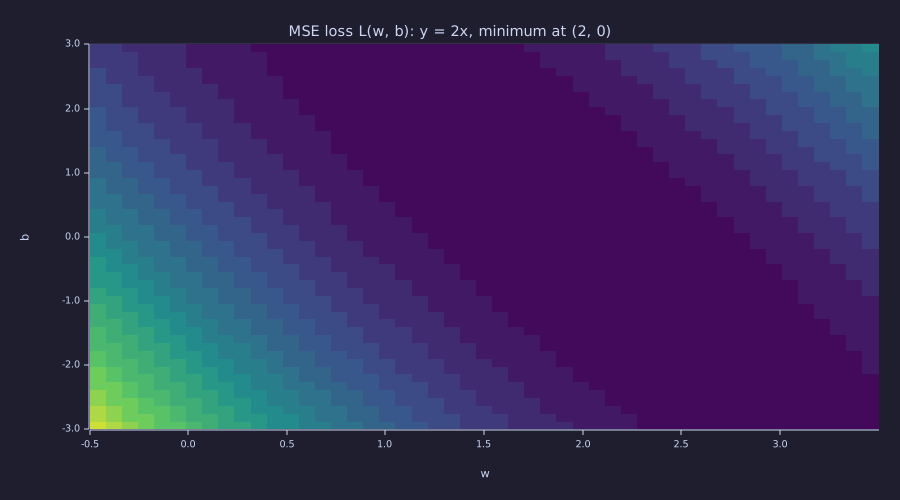
The dark trough runs diagonally from upper-left to lower-right with slope \(\approx -3\): that is the slow eigenvector. Bands are far apart along it and crowd together across it — low curvature along the valley, high curvature across it.
Analytic check: \(\mathcal{L}(2, 0) = 0.000\) from the expanded formula. The minimum over the \(50 \times 50\) grid is \(0.0014\) — a hair above zero because the grid doesn't land exactly on \((2, 0)\).
Gradient Descent
Theory
The gradient \(\nabla \mathcal{L} = [\partial \mathcal{L}/\partial w,\; \partial \mathcal{L}/\partial b]\) points toward steepest ascent. We move in the opposite direction:
\[w \leftarrow w - \eta \frac{\partial \mathcal{L}}{\partial w}, \qquad b \leftarrow b - \eta \frac{\partial \mathcal{L}}{\partial b},\]
where \(\eta > 0\) is the learning rate. To find the partial derivatives, start from the loss written out explicitly:
\[\mathcal{L}(w, b) = \frac{1}{N} \sum_{i=1}^{N} (w x_i + b - y_i)^2.\]
Differentiate term by term. The chain rule on each square pulls down a factor of \(2\) times the inside, times the derivative of the inside with respect to the parameter. That inner derivative is \(x_i\) for \(w\) and \(1\) for \(b\):
\[\frac{\partial \mathcal{L}}{\partial w} = \frac{1}{N} \sum_{i=1}^{N} 2 (w x_i + b - y_i)\, x_i, \qquad \frac{\partial \mathcal{L}}{\partial b} = \frac{1}{N} \sum_{i=1}^{N} 2 (w x_i + b - y_i)\, (1).\]
Factor the constant \(2/N\) out of each sum and write \(\hat{y}_i = w x_i + b\):
\[\frac{\partial \mathcal{L}}{\partial w} = \frac{2}{N} \sum_{i=1}^{N} (\hat{y}_i - y_i) \cdot x_i, \qquad \frac{\partial \mathcal{L}}{\partial b} = \frac{2}{N} \sum_{i=1}^{N} (\hat{y}_i - y_i).\]
For a quadratic this is the same as \(\nabla \mathcal{L} = \mathbf{H}\,\mathbf{e}\) — the gradient is the Hessian times the current error — which is the fact the Systems lens turns into a stability theory.
Example — 200 steps from (0, 0) at η = 0.05
lr = 0.05;
n_steps = 200;

w = 0.0;
b = 0.0;

w_path    = zeros(n_steps + 1);
b_path    = zeros(n_steps + 1);
loss_path = zeros(n_steps + 1);

w_path(1)    = w;
b_path(1)    = b;
loss_path(1) = mean((w * x + b - y) .^ 2);

for step = 1:n_steps
  pred     = w * x + b;
  residual = pred - y;
  dw = (2.0 / npts) * sum(residual .* x);
  db = (2.0 / npts) * sum(residual);
  w -= lr * dw;
  b -= lr * db;
  w_path(step + 1)    = w;
  b_path(step + 1)    = b;
  loss_path(step + 1) = mean((w * x + b - y) .^ 2);
end
print("after", n_steps, "steps: w =", w, " b =", b, " loss =", loss_path(n_steps + 1));after 200 steps: w = 1.9898446957772915 b = 0.029857832820454414 loss = 0.00014888983103998946After 200 steps with \(\eta = 0.05\): \(w = 1.9898\) (true \(w^* = 2\)), \(b = 0.0299\) (true \(b^* = 0\)), \(\mathcal{L} = 1.49e-04\). That is small, but it is not converged, and the Hessian says exactly why. In the eigenbasis the two error components decay independently, each by its own factor \(1 - \eta\lambda_i\) per step (derived in the Systems lens): the fast mode by \(1 - 0.05 \times 16.70 = 0.165\) — gone within five steps — and the slow mode by \(1 - 0.05 \times 0.299 = 0.985\), so after 200 steps \(0.049\) of it remains: 5 % of the initial slow-mode error. The remaining error should therefore point along the slow eigenvector with that length:
e0   = [0.0 - 2.0; 0.0 - 0.0];                          % initial error (w - w*, b - b*)
coef = V' * e0;                                          % modal coordinates of e0
rho_slow = 1.0 - lr * lam_slow;
e_pred = v_slow * (coef(i_slow) * rho_slow ^ n_steps);   % slow mode alone, 200 steps on
print("slow-mode pole =", rho_slow, "   rho^200 =", rho_slow ^ n_steps);
print("predicted error (slow mode only) =", [e_pred(1), e_pred(2)]);
print("actual error (w - 2, b) =", [w - 2.0, b]);slow-mode pole = 0.9850304866714181 rho^200 = 0.04897048688929904
predicted error (slow mode only) = [1×2] -0.010155 0.029858
actual error (w - 2, b) = [1×2] -0.010155 0.029858The prediction matches the actual error to four decimals: the fast mode contributes \(3.0e-157\) of its start, nothing. The path has been crawling along the valley floor for 195 of its 200 steps. The slow mode's time constant is \(-1/\ln 0.985 \approx 66\) steps, so reaching \(10^{-6}\) of the initial error would take about \(916\) steps at this learning rate.
Example — Loss vs. step
On a log axis a geometric decay is a straight line, and this run has two of them.
steps  = 0:n_steps;
L_slow = 0.5 * lam_slow * (coef(i_slow) * rho_slow .^ steps) .^ 2;   % the slow mode's share of the loss

figure();
hold("on")
semilogy(steps, loss_path, "color", "blue", "label", "MSE loss")
semilogy(steps, L_slow, "color", "red", "label", "slow mode only (dashed)", "style", "dashed")
title("Gradient descent at eta = 0.05: two decay regimes")
xlabel("step k")
ylabel("MSE loss (log scale)")
legend()
hold("off")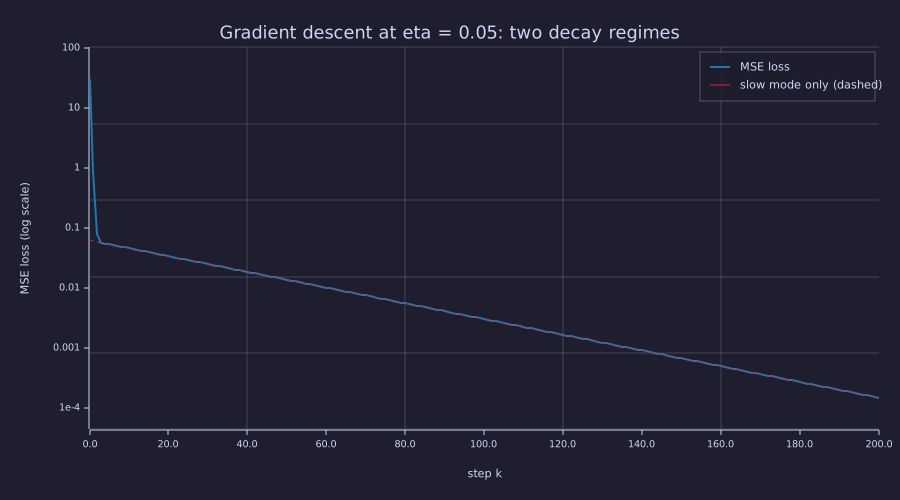
The first five steps drop the loss by two decades at the fast pole's rate; from then on the blue curve lies exactly on the dashed slow-mode line, whose slope is \(2 \ln 0.985\) per step. "Converged" on a linear axis, still decaying on a log axis.
Example — Trajectory in (w, b) space
The level sets of \(\mathcal{L}\) are ellipses on the Hessian eigenvectors, so they can be drawn in closed form and the path laid over them.
phi = linspace(0, 2 * pi, 100);
figure();
hold("on")
for c = [0.03, 0.3, 3.0, 30.0]
  ew = 2.0 + v_fast(1) * sqrt(2 * c / lam_fast) * cos(phi) + v_slow(1) * sqrt(2 * c / lam_slow) * sin(phi);
  eb =       v_fast(2) * sqrt(2 * c / lam_fast) * cos(phi) + v_slow(2) * sqrt(2 * c / lam_slow) * sin(phi);
  plot(ew, eb, "color", "gray", "label", sprintf("L = %g", c))
end
plot([2 - 2 * v_slow(1), 2 + 2 * v_slow(1)], [-2 * v_slow(2), 2 * v_slow(2)], "color", "green", "label", "slow eigenvector", "style", "dashed")
plot([2 - 0.5 * v_fast(1), 2 + 0.5 * v_fast(1)], [-0.5 * v_fast(2), 0.5 * v_fast(2)], "color", "orange", "label", "fast eigenvector", "style", "dashed")
plot(w_path, b_path, "color", "red", "label", "GD path, eta = 0.05")
scatter(w_path(1:3), b_path(1:3), "color", "red", "label", "steps 0, 1, 2")
xlim([-0.5, 3.5])
ylim([-3.0, 3.0])
title("GD path over the level-set ellipses of L(w, b)")
xlabel("w")
ylabel("b")
legend()
hold("off")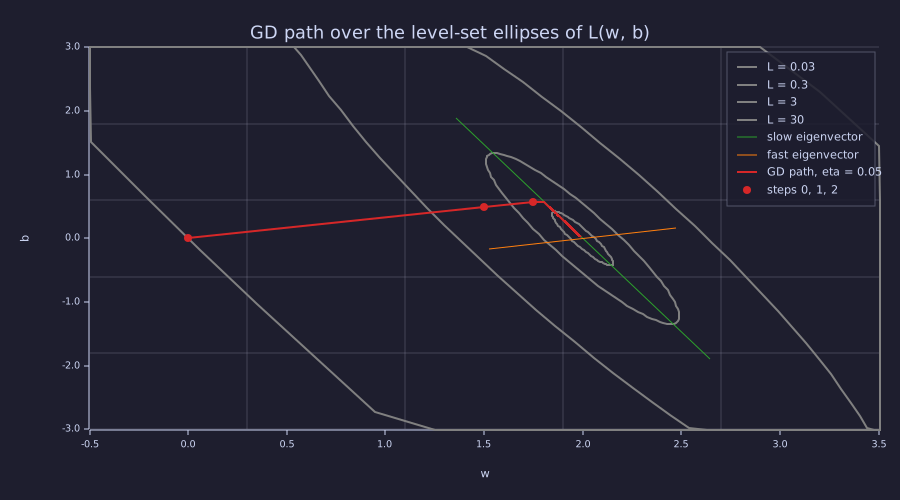
One step takes the path from \((0, 0)\) to \((1.5, 0.5)\) — almost all of the fast-mode error — then it turns onto the green valley floor and crawls toward \((2, 0)\) without reaching it in 200 steps. The "curve" is one sharp bend, not a smooth arc.
Learning Rate Sensitivity
Theory
| \(\eta\) | Behaviour |
|---|---|
| Too large | Overshoots the minimum; loss oscillates or diverges |
| Too small | Convergence is slow; many iterations needed |
| Well-chosen | Loss decreases smoothly to the minimum |
The threshold between the rows is not a matter of taste: it is \(\eta < 2/\lambda_{\max} = 0.1198\) for this problem, derived in the Systems lens below, where the three rows become three pole locations.
Example — One step verified by hand
- Initial: \(w_0 = 0\), \(b_0 = 0\), predictions \(= [0,0,0,0]\), residuals \(= [-2,-4,-6,-8]\).
- \(\partial \mathcal{L}/\partial w = 0.5 \times ((-2)(1) + (-4)(2) + (-6)(3) + (-8)(4)) = -30\).
- \(\partial \mathcal{L}/\partial b = 0.5 \times (-2-4-6-8) = -10\).
- \(w_1 = 0 - 0.05 \times (-30) = 1.5,\;\; b_1 = 0 - 0.05 \times (-10) = 0.5\).
These match the second entries w_path(2) / b_path(2) from the descent loop above — entry 1 holds the initial \((0, 0)\), and entry 2 is the state after the first update.
The Bigram Model as a Linear Layer
Theory
Lesson 05 estimated \(P(x_{t+1} \mid x_t)\) by counting. The same model is a linear layer with a one-hot input: take \(\mathbf{W} \in \mathbb{R}^{|\mathcal{V}| \times |\mathcal{V}|}\), feed the one-hot of the current token \(\mathbf{e}_i\), and read the logits \(\mathbf{z} = \mathbf{e}_i \mathbf{W} = \mathbf{W}_{i,:}\) — row \(i\) of \(\mathbf{W}\). Softmax of that row is the model's \(\hat{\mathbf{p}}(\cdot \mid i)\), and the training loss is Lesson 03's cross-entropy averaged over the \(N\) bigrams of the corpus. Grouping the bigrams by their current token, with \(C_{ij}\) the count matrix and \(n_i = \sum_j C_{ij}\),
\[\mathcal{L}(\mathbf{W}) = -\frac{1}{N}\sum_{i,j} C_{ij} \log \mathrm{softmax}(\mathbf{W}_{i,:})_j.\]
Its gradient is Lesson 03's error signal, one row at a time, weighted by how often that row occurs:
\[\frac{\partial \mathcal{L}}{\partial \mathbf{W}_{i,:}} = \frac{n_i}{N}\Bigl(\mathrm{softmax}(\mathbf{W}_{i,:}) - \mathbf{P}_{i,:}\Bigr), \qquad \mathbf{P}_{i,:} = \mathbf{C}_{i,:} / n_i,\]
because summing \(\hat{\mathbf{p}} - \mathbf{y}\) over the \(n_i\) bigrams that start at \(i\) replaces the one-hot targets by their average, the empirical row \(\mathbf{P}_{i,:}\). The gradient vanishes exactly when \(\mathrm{softmax}(\mathbf{W}_{i,:}) = \mathbf{P}_{i,:}\), i.e. when
\[W_{ij} = \log P_{ij} + c_i\]
for any per-row constant \(c_i\) (softmax is shift-invariant). Gradient descent on the linear layer therefore converges to the same optimum the count estimator finds in closed form — "learn" and "look up" agree — and the loss it converges to is Lesson 05's conditional entropy \(H(X_{t+1} \mid X_t)\). Where \(P_{ij} = 0\) the optimum sits at \(W_{ij} \to -\infty\): the asymptotic floor of Lesson 03's loss surface, approached but never reached.
Example — Training the bigram layer on "abcbabcba"
seq = [1, 2, 3, 2, 1, 2, 3, 2, 1];          % "abcbabcba", a=1 b=2 c=3 (Lesson 05)
vocab_size = 3;
C = zeros(vocab_size, vocab_size);
for t = 1:(length(seq) - 1)
  C(seq(t), seq(t + 1)) = C(seq(t), seq(t + 1)) + 1;
end
n_row = sum(C, 2);                            % bigrams starting at each token
N_big = sum(n_row);
P = C ./ n_row;                               % Lesson 05's count estimator

W_bi = zeros(vocab_size, vocab_size);         % all logits equal: uniform rows
lr_bi = 2.0;
n_bi = 300;
loss_bi = zeros(n_bi);
for k = 1:n_bi
  P_hat = softmax(W_bi);                      % row-wise softmax: one-hot . W for every row at once
  G = (n_row .* P_hat - C) / N_big;           % (n_i / N) (p_hat_i - P_i), row by row
  W_bi = W_bi - lr_bi * G;
  loss_bi(k) = -sum(sum(C .* log(softmax(W_bi)))) / N_big;
end
print("softmax(W) after", n_bi, "steps ="); print(softmax(W_bi));
print("count estimator P ="); print(P);
print("loss:", loss_bi(1), "->", loss_bi(n_bi), "nats;   H(X_t+1 | X_t) =", log(2) / 2, "nats");
print("row b logits:", W_bi(2, :), " W_ba - W_bc =", W_bi(2, 1) - W_bi(2, 3), "= log(P_ba / P_bc)");softmax(W) after 300 steps =
Matrix(3x3)
[0.002249, 0.995502, 0.002249]
[0.498892, 0.002215, 0.498892]
[0.002249, 0.995502, 0.002249]
count estimator P =
Matrix(3x3)
[0.000000, 1.000000, 0.000000]
[0.500000, 0.000000, 0.500000]
[0.000000, 1.000000, 0.000000]
loss: 0.8761984286823383 -> 0.3499364930370649 nats; H(X_t+1 | X_t) = 0.34657359027997264 nats
row b logits: [1×3] 1.805701 -3.611401 1.805701 W_ba - W_bc = 0 = log(P_ba / P_bc)Lesson 05 printed \(0.3466\) nats as the cross-entropy of \(\mathbf{P}\) on this corpus; after 300 steps the layer is at \(0.3499\) nats, within \(0.0034\) of it, and \(\mathrm{softmax}(\mathbf{W})\) matches \(\mathbf{P}\) to two decimals. Row \(b\) — the one row with no zero counts — has converged exactly: \(W_{ba} - W_{bc} = 0.0000 = \log(0.5 / 0.5)\). Rows \(a\) and \(c\) keep pushing their two zero-count logits toward \(-\infty\) and account for the whole remaining gap.
Engineering Lenses
Gradient descent on a quadratic is not like a linear discrete-time system — it is one, so the Systems lens here is exact and carries the lesson's main result. No signals reading adds to this lesson: the only signal is the four-sample residual, and nothing filters it yet (momentum will, in 16-adamw-optimizer).
Systems
Exact. Substitute the gradient \(\nabla \mathcal{L} = \mathbf{H}(\boldsymbol{\theta} - \boldsymbol{\theta}^*)\) of a quadratic into the update \(\boldsymbol{\theta}_{k+1} = \boldsymbol{\theta}_k - \eta \nabla \mathcal{L}\) and subtract \(\boldsymbol{\theta}^*\) from both sides:
\[\mathbf{e}_{k+1} = (\mathbf{I} - \eta \mathbf{H})\, \mathbf{e}_k .\]
This is an autonomous linear time-invariant system: state \(\mathbf{e}_k\) (the parameter error), state matrix \(\mathbf{A} = \mathbf{I} - \eta\mathbf{H}\), no input. In the eigenbasis of \(\mathbf{H}\) it decouples into scalar modes \(c_{i,k+1} = (1 - \eta\lambda_i)\, c_{i,k}\), so the poles are
\[z_i = 1 - \eta \lambda_i, \qquad \mathbf{e}_k = \sum_i c_{i,0}\, z_i^{\,k}\, \mathbf{v}_i .\]
Discrete-time stability requires every pole inside the unit circle, \(|1 - \eta\lambda_i| < 1\), i.e. \(0 < \eta < 2/\lambda_i\) for every \(i\):
\[\boxed{\;\eta < \frac{2}{\lambda_{\max}}\;}\]
Each mode has time constant \(\tau_i = -1/\ln|z_i|\) steps: the slowest mode sets the settling time, the stiffest sets the stability limit, and their ratio \(\kappa\) is why no single \(\eta\) serves both — the best fixed step, \(\eta^* = 2/(\lambda_{\max} + \lambda_{\min})\), still leaves both poles at magnitude \((\kappa - 1)/(\kappa + 1)\). A pole in \((0, 1)\) decays monotonically; one in \((-1, 0)\) decays while flipping sign every step (the zig-zag across the valley); one beyond \(-1\) grows. 16-adamw-optimizer and 17-learning-rate-scheduling reuse this bound: momentum moves the poles, a schedule makes them time-varying.
eta_crit = 2.0 / lam_fast;
eta_star = 2.0 / (lam_fast + lam_slow);
print("stability limit 2/lambda_max =", eta_crit, "   best fixed step =", eta_star, "  (pole magnitude", (kappa - 1) / (kappa + 1), ")");
etas = [0.05, 0.10, 0.12, 0.20];
for i = 1:length(etas)
  poles = 1.0 - etas(i) * [lam_fast, lam_slow];
  print("eta =", etas(i), "   poles =", poles, "   tau_slow =", -1.0 / log(abs(poles(2))), "steps");
end

A_gd = eye(2) - lr * H;
e_k  = e0;
for k = 1:n_steps
  e_k = A_gd * e_k;             % (I - eta H)^k e0 by repeated multiplication (A^k is element-wise in rustlab)
end
print("(I - eta H)^200 e0 =", [e_k(1), e_k(2)], " GD's actual error =", [w - 2.0, b]);stability limit 2/lambda_max = 0.11975610662865495 best fixed step = 0.11764705882352941 (pole magnitude 0.9647776156974546 )
eta = 0.05 poles = [1×2] 0.164970 0.985030 tau_slow = 66.30118204786606 steps
eta = 0.1 poles = [1×2] -0.670061 0.970061 tau_slow = 32.8986864766667 steps
eta = 0.12 poles = [1×2] -1.004073 0.964073 tau_slow = 27.33130061650427 steps
eta = 0.2 poles = [1×2] -2.340122 0.940122 tau_slow = 16.195464586885233 steps
(I - eta H)^200 e0 = [1×2] -0.010155 0.029858 GD's actual error = [1×2] -0.010155 0.029858At \(\eta = 0.05\) the poles are \(0.165\) and \(0.985\) — the two slopes of the loss curve above — and iterating \(\mathbf{I} - \eta\mathbf{H}\) two hundred times reproduces the descent loop's final error exactly. At \(\eta = 0.10\) the fast pole crosses to \(-0.670\): still stable, but \(w\) now overshoots the valley on every step. At \(\eta = 0.12\) it sits at \(-1.004\), just outside the circle, and at \(0.20\) at \(-2.34\).
theta = linspace(0, 2 * pi, 200);
pole_cols = {"blue", "green", "orange", "red"};
figure();
hold("on")
plot(cos(theta), sin(theta), "color", "gray", "label", "unit circle")
for i = 1:length(etas)
  poles = 1.0 - etas(i) * [lam_fast, lam_slow];
  scatter(poles, [0.0, 0.0], "color", pole_cols(i), "label", sprintf("eta = %.2f", etas(i)))
end
axis("equal")
xlim([-2.5, 1.5])
ylim([-1.2, 1.2])
title("Poles 1 - eta lambda_i of the GD error system")
xlabel("Re z")
ylabel("Im z")
legend()
hold("off")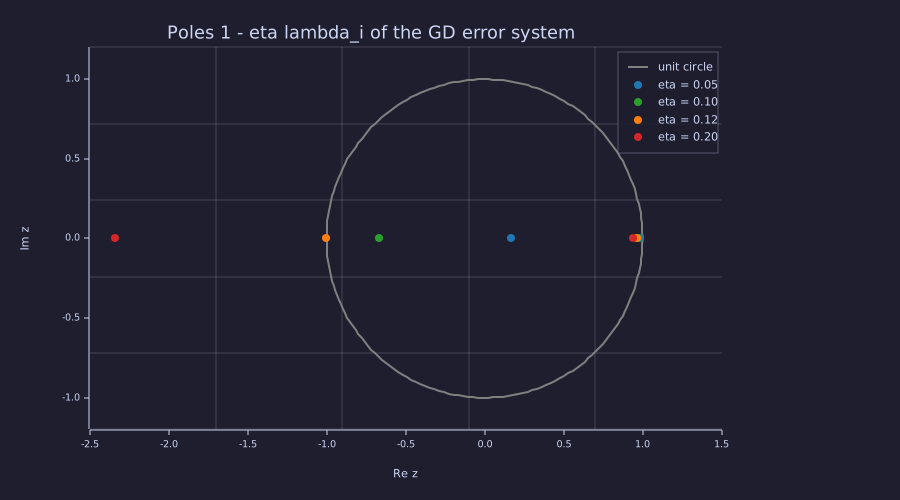
Each colour is one learning rate and has two dots: the slow pole hugging \(+1\) (it barely moves with \(\eta\)) and the fast pole marching left through \(0\), past \(-1\) at \(\eta = 0.12\), and off to \(-2.3\). Stability is lost by the fast mode while the slow mode is still crawling.
The three regimes, run for 25 steps each. Because the loss is a sum of squared modal errors it decays monotonically whenever the run is stable — it cannot see a sign flip — so the bottom row plots the fast-mode coordinate \(c_{\text{fast},k} = \mathbf{v}_{\text{fast}}^\top \mathbf{e}_k\) itself.
function [loss_hist, c_fast] = gd_run(x, y, eta, n_steps, v_fast)
  w = 0.0; b = 0.0; npts = length(x);
  loss_hist = zeros(n_steps + 1); c_fast = zeros(n_steps + 1);
  loss_hist(1) = mean((w * x + b - y) .^ 2);
  c_fast(1) = v_fast(1) * (w - 2.0) + v_fast(2) * b;
  for k = 1:n_steps
    r  = w * x + b - y;
    w -= eta * (2.0 / npts) * sum(r .* x);
    b -= eta * (2.0 / npts) * sum(r);
    loss_hist(k + 1) = mean((w * x + b - y) .^ 2);
    c_fast(k + 1) = v_fast(1) * (w - 2.0) + v_fast(2) * b;
  end
end

etas3 = [0.05, 0.10, 0.20];
cols3 = {"blue", "green", "red"};
k25 = 0:25;
figure();
for j = 1:3
  [L_run, c_run] = gd_run(x, y, etas3(j), 25, v_fast);
  print("eta =", etas3(j), "  loss after 25 steps =", L_run(26), "  fast-mode error, steps 0-3 =", c_run(1:4));
  subplot(2, 3, j)
  semilogy(k25, L_run, "color", cols3(j), "label", "loss")
  title(sprintf("eta = %.2f: loss", etas3(j)))
  subplot(2, 3, 3 + j)
  hold("on")
  plot(k25, c_run, "color", cols3(j), "label", "fast-mode error c_fast")
  hline(0.0, "gray", "0")
  xlabel("step")
  hold("off")
endeta = 0.05 loss after 25 steps = 0.029206519013275662 fast-mode error, steps 0-3 = [1×4] -1.893475 -0.312366 -0.051531 -0.008501
eta = 0.1 loss after 25 steps = 0.013581563460824012 fast-mode error, steps 0-3 = [1×4] -1.893475 1.268744 -0.850136 0.569643
eta = 0.2 loss after 25 steps = 86725340321479300000 fast-mode error, steps 0-3 = [1×4] -1.893475 4.430963 -10.368993 24.264708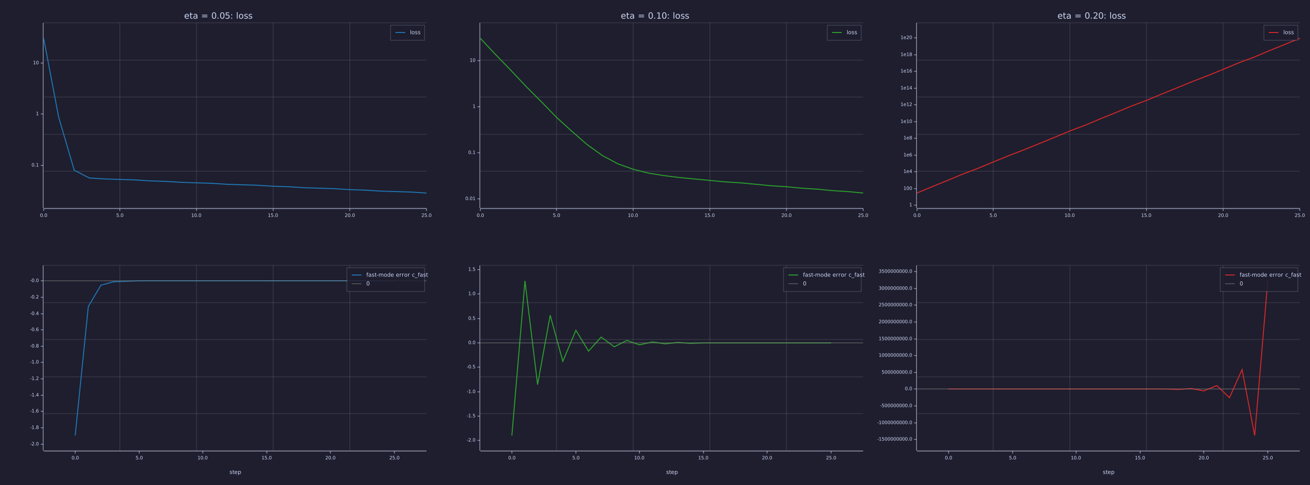
Top row (poles \(0.165\) / \(-0.670\) / \(-2.34\) for the fast mode): monotone, monotone, diverging — the loss hides the oscillation. Bottom row: the fast-mode error decays smoothly at \(\eta = 0.05\), alternates sign every step while shrinking at \(\eta = 0.10\), and alternates while growing \(2.34\times\) per step at \(\eta = 0.20\).
Exact. The vector field \(-\nabla \mathcal{L} = -\mathbf{H}\mathbf{e}\) is the flow the update follows; drawn over the contours it shows why the path bends.
w_q = linspace(-0.5, 3.5, 9);
b_q = linspace(-3.0, 3.0, 13);
[W_q, B_q] = meshgrid(w_q, b_q);
U_q = -(H(1, 1) * (W_q - 2.0) + H(1, 2) * B_q);     % -dL/dw
V_q = -(H(2, 1) * (W_q - 2.0) + H(2, 2) * B_q);     % -dL/db
figure();
hold("on")
contour(W_mesh, B_mesh, L_matrix, [0.03, 0.3, 3.0, 30.0])
quiver(W_q, B_q, U_q, V_q)
title("-grad L = -H (theta - theta*): the flow gradient descent follows")
xlabel("w")
ylabel("b")
hold("off")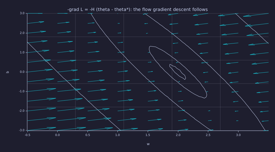
Almost every arrow points across the valley, not along it: the field is dominated by the stiff eigenvector (\(\lambda = 16.7\)). Only on the two eigenvector lines through \((2, 0)\) does an arrow point straight at the minimum; everywhere else gradient descent first slams into the valley floor and then turns.
Model. As a block diagram, gradient descent is a feedback loop whose only dynamic element is an integrator — the parameter memory — with loop gain \(\eta\mathbf{H}\) and closed-loop poles \(1 - \eta\lambda_i\). Later lessons change one block at a time: 15-backpropagation computes the gradient block for any network, 16-adamw-optimizer puts a filter (momentum) and a per-coordinate gain (Adam) in the gradient path, 17-learning-rate-scheduling schedules \(\eta\), and 18-training-loop adds the noisy minibatch sensor and a limiter.
Information
Exact. The bigram layer's loss cannot go below Lesson 05's conditional entropy, and it gets there. The floor is \(H(X_{t+1} \mid X_t) = \sum_i \pi_i H(\mathbf{P}_{i,:})\) with \(\pi_i = n_i / N\) the frequency of the current token. A one-hot input carries no information beyond the identity of the current token, so no linear layer — indeed no function of \(x_t\) alone — can do better than the count table; gradient descent simply approaches the same bound from the uniform start \(\log_2 |\mathcal{V}| = 1.585\) bits.
H_rows  = row_entropies_bits(P);                 % bits per row of the count estimator
pi_cur  = n_row' / N_big;                        % frequency of the current token
floor_bits = sum(pi_cur * H_rows');              % H(X_t+1 | X_t) = sum_i pi_i H(P_i,:)
print("row entropies (bits):", H_rows, "   pi =", pi_cur);
print("conditional-entropy floor =", floor_bits, "bits =", floor_bits * log(2), "nats");
print("linear layer after", n_bi, "steps:", loss_bi(n_bi) / log(2), "bits   gap =", loss_bi(n_bi) / log(2) - floor_bits, "bits");

figure();
hold("on")
loss_curve = [log(3.0), loss_bi];               % step 0 = uniform logits (loss log|V|); loss_bi(k) is logged after update k
plot(0:n_bi, loss_curve / log(2), "color", "blue", "label", "bigram linear layer, GD")
hline(floor_bits, "red", "H(X_t+1 | X_t) = 0.5 bit")
hline(log2(3), "gray", "log2 |V| = uniform start")
title("Cross-entropy of the learned bigram layer vs. the conditional-entropy floor")
xlabel("gradient step")
ylabel("cross-entropy (bits / token)")
legend()
hold("off")row entropies (bits): [1×3] 0.000000 1.000000 0.000000 pi = Matrix(1x3)
[0.250000, 0.500000, 0.250000]
conditional-entropy floor = 0.5 bits = 0.34657359027997264 nats
linear layer after 300 steps: 0.5048516431306489 bits gap = 0.004851643130648897 bits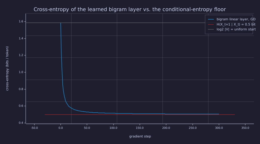
The curve starts on the grey line at \(\log_2 3 = 1.585\) bits (step 0, uniform logits), falls toward the red floor, and flattens \(0.005\) bit above it: gradient descent rediscovers the count table's \(0.5\) bit per token, and nothing that sees only the current token can go lower.
Key Takeaways
- A linear layer is \(\mathbf{y} = \mathbf{x}\mathbf{W} + \mathbf{b}\) with \(\mathbf{W} \in \mathbb{R}^{d_{\text{in}} \times d_{\text{out}}}\); every component of a language model is one, or a composition of them with non-linear activations.
- Gradient descent on a quadratic is the LTI system \(\mathbf{e}_{k+1} = (\mathbf{I} - \eta\mathbf{H})\mathbf{e}_k\): poles \(1 - \eta\lambda_i\), stable iff \(\eta < 2/\lambda_{\max}\) (\(0.1198\) here). The condition number \(\kappa = 55.8\) is why 200 steps still leave 5 % of the slow-mode error.
- The valley is the slow eigenvector, not "the \(b\) axis": the path takes one step across it and then crawls along it.
- The bigram model is a \(|\mathcal{V}| \times |\mathcal{V}|\) linear layer; gradient descent drives it to \(W_{ij} = \log P_{ij} + c_i\) and to the \(0.5\)-bit conditional-entropy floor — "learn" and "look up" agree.
- Stacking linear layers without non-linearity is still one linear layer; the activation function (11-feed-forward-block) is what makes deep networks expressive.
Standalone Scripts
| Script | What it computes |
|---|---|
loss_landscape.rlab | the Hessian, its eigenvalues / eigenvectors and \(\kappa\); filled contours of \(\mathcal{L}(w, b)\) on real axes |
gradient_descent.rlab | 200 steps at \(\eta = 0.05\); the slow-mode prediction of the remaining error; semilogy loss with the slow-mode line; the path over the level-set ellipses |
gd_stability.rlab | poles \(1 - \eta\lambda_i\) for four learning rates on the unit circle; the monotone / oscillating / diverging runs; the \(-\nabla\mathcal{L}\) flow field |
bigram_linear_layer.rlab | the bigram model as a \(\lvert\mathcal{V}\rvert \times \lvert\mathcal{V}\rvert\) linear layer trained by gradient descent; convergence to \(\mathbf{P}\) and to the \(0.5\)-bit floor |
Run all with make lesson-06 (or rustlab run lessons/06-linear-layers-and-gradient-descent/<name>.rlab).
Expected Numerical Outputs Summary
| Variable | Expected Value |
|---|---|
L_true (= \(\mathcal{L}(2, 0)\)) | 0.000 |
L_init (= \(\mathcal{L}(0, 0)\)) | 30.0 |
lam_fast, lam_slow | 16.70, 0.2994 |
kappa | ≈ 55.8 |
L_check (analytic) | 0.000 |
min_loss_flat (over the 50 × 50 grid) | ≈ 0.0014 |
Final w, b after 200 steps | 1.9898, 0.0299 (not converged) |
Final loss_path(end) | ≈ 1.49e-04 |
rho_slow, rho_slow^200 | 0.9850, 0.0490 |
e_pred = actual error | ≈ [-0.0102, 0.0299] |
| Step-1 hand check \(w_1\), \(b_1\) | 1.5, 0.5 |
eta_crit (= \(2/\lambda_{\max}\)), eta_star | 0.1198, 0.1176 |
| Poles at \(\eta = 0.05 / 0.10 / 0.12 / 0.20\) (fast) | 0.165 / -0.670 / -1.004 / -2.340 |
loss_bi(1) → loss_bi(300) | 0.876 → 0.3499 nats (floor 0.3466) |
floor_bits | 0.5 bits |
Exercises
- Predict, then run. Using the poles, predict what happens at \(\eta = 0.11\) and at \(\eta = 0.15\) before running
gd_stability.rlabwith those values. At what learning rate would the slow pole leave the unit circle, and why is that number irrelevant in practice? - Gradient at the minimum. At \((w^*, b^*) = (2, 0)\), compute \(\partial \mathcal{L}/\partial w\) and \(\partial \mathcal{L}/\partial b\) by hand. Confirm both are zero, and confirm \(\nabla \mathcal{L} = \mathbf{H}\mathbf{e}\) at \((0, 0)\) reproduces \((-30, -10)\).
- Non-zero bias. Change the dataset to \(y = [3, 5, 7, 9]\) (true relationship \(y = 2x + 1\)). Re-run
gradient_descent.rlab. Where does the algorithm converge? Does \(\mathbf{H}\) — and therefore \(\kappa\) and the stability limit — change? - Counting parameters. A language model uses a linear layer to project from embedding dimension \(d = 512\) to vocabulary size \(|\mathcal{V}| = 50{,}000\). How many parameters does this output linear layer have (weights + biases)? What fraction of GPT-2-small's 117M parameters does this represent?
- The best fixed step. Set \(\eta = \eta^* = 2/(\lambda_{\max} + \lambda_{\min})\). What are the two poles? How many steps does it take to bring the slow-mode error to \(10^{-6}\) of its start, compared with \(\eta = 0.05\)?
What's next
07-context-and-naive-averaging returns to the language-modelling thread: it gives the bigram model more context by averaging the embedding vectors of all tokens seen so far — the simplest form of attention. This sets up 08-scaled-dot-product-attention, which replaces the uniform average with learned attention weights computed from queries, keys, and values. The gradient itself is generalised to arbitrary compositions of layers in 15-backpropagation, and the feedback loop drawn above is refined block by block in Lessons 16–18.